| Date: | March 20/21 |
| Lecture: | 26 |
| Homework | HW #12 |
| Excel: | lecture26.xlsx |
| Status: | In Progress |
| Handout: | Hand26.docx |
| Code: | Filter Block Demo XDC file Support pack |
| Lesson Slides | ECE_383_Lec26.pptx |
Digital Filter in Theory
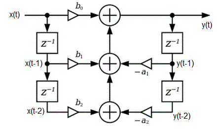
In today's class we will be building filters. Our filters are called Infinite Impulse Response filter (IIR) because if they are given an impulse as an input signal, it will "ring" forever (i.e., have an infinite impulse response). From within this broad class of filters, we will be examining Biquadratic so names because the system function consists of two quadratic equations.You can build a digital version of the analog filters we discussed last lecture. The process of calculating a filtered output y(t) is described by the following imaged, a slightly modified version that I copied from the Wikipedia page on Digital Biquad Filters.

Some comments are in order.
- The input stream of digitized inputs is described by x(t). The blocks labeled "z-1" is a delay block. We will call the nodes below each of the blocks on the left side as x(t-1) and x(t-2), in order to indicate that they are 1 and 2 time units older than x(t). Note that x(t-2) will get the value of x(t-1), in 1 time unit from now. Likewise y(t-1) and y(t-2) are the old outputs 1 and 2 time units ago.
- The triangles are multipliers, the two inputs to the multiplier are the input to the triangle and the variable above or below.
- The circles with "+" inside of them are adders.
output y(t) = x(t)*b0 + x(t-1)*b1 + x(t-2)*b2 - y(t-1)*a1 - y(t-2)*a2Since the inputs x(t) are given, and the y(t)'s are found, then in order to build this filter, we will need to know the coefficients a2, a1, b2, b1, b0. Since this is not a course in digital signal processing, we will use cookbook equations to derive these values found in the excel file linked at the top of this file.
Digital Filter in Excel
In order to better understand how these filters operate, I've provided excel file at the top of this page which contains three tabs. Each of these tabs is explained in the sections below.Second Order tab
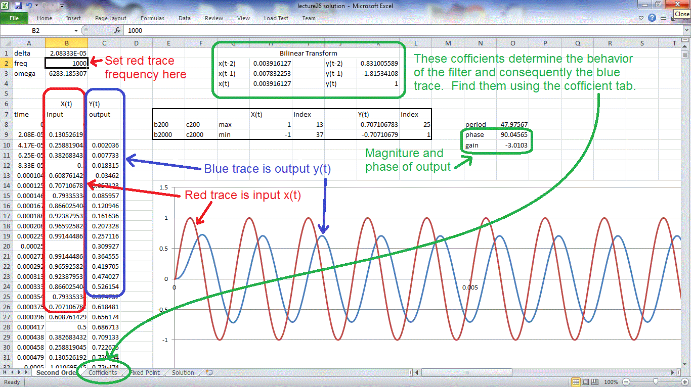
The image below shows the major features of this tab. The frequency of the input sinusoid is set by cell B2. The amplitude of the sinusoid is calculated in column B8:B2000 and displayed as the red trace in the graph. The filter is defined by the coefficients in the green rectangle H2:H4 and K2:K4. You will need to use the coefficients tab to determine these values. The output values, compute in column C8:C2000 are plotted as the blue trace in the graph.
Coefficient tab
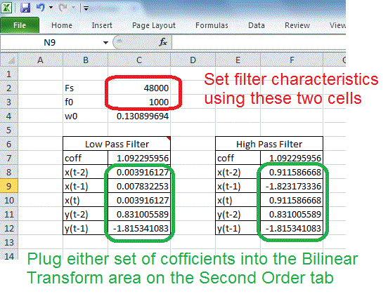
The coefficients tab allows you to specify the behavior of the filter by specifying the corner frequency (denoted f0 in cell C3) and the sampling frequency (denoted Fs in cell C2). I've provided two calculators, one for low-pass filter and one for high-pass filter. Choose which ever set you want to copy into appropriate cells in the Second Order tab.
Fixed Point tab
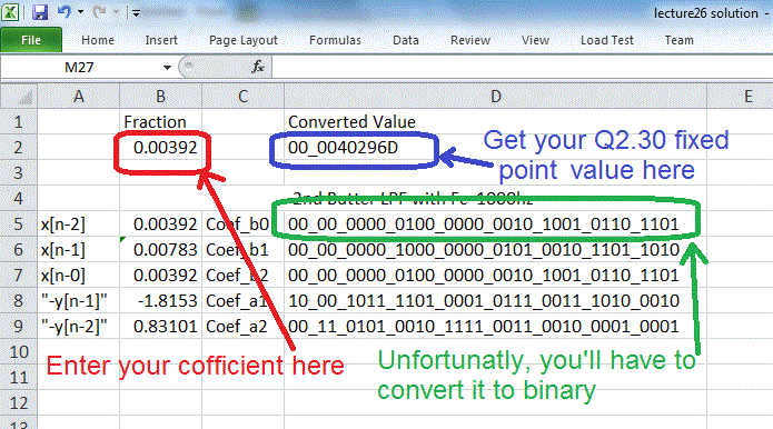
In order to build the BiQuad filter in VHDL, you will need to specify the coefficients using a fixed point representation. So I created a handy tab to do just that. Plug in your signed decimal value in the range [-2 to +1.99999] and you will get the Q2.30 fixed point representation in blue. I was too lazy to write an expression to convert it to binary, so you will just have to do that part by hand to get the values in green.
You may be asking yourself, how do I use these coefficients to build a digital filter in VHDL? We read-on my intrepid friend.
Digital Filter in VHDL
I borrowed code from eewiki for the filter linked at the top of this web page. The filter is general enough to accomodiate any filter specified by the cofficients used in the excel file. the code snippet below show the component instantiation of a filter block realizing a low pass filter with cutoff frequency of 1000Hz.------------------------------------------------------------------ -- Low pass 2nd order butterworth filter with -- f0 = 1000Hz, Fs = 48000Hz ------------------------------------------------------------------ left_filter_lpf500: entity work.IIR_Biquad(arch) generic map( Coef_b0 => B"00_00_0000_0100_0000_0010_1001_0110_1101", -- +0.003916127 Coef_b1 => B"00_00_0000_1000_0000_0101_0010_1101_1010", -- +0.007832253 Coef_b2 => B"00_00_0000_0100_0000_0010_1001_0110_1101", -- +0.003916127 Coef_a1 => B"10_00_1011_1101_0001_0111_0011_1010_0010", -- -1.815341083 Coef_a2 => B"00_11_0101_0010_1111_0011_0010_0001_0001") -- +0.831005589 port map ( clk => clk, -- Normal 100Mhz clock n_reset => reset, -- Our normal active low reset sample_trig => ready, -- This is the ready signal from the AC'97 wrapper X_in => Ladc, -- The adc output from the ac'97 wrapper filter_done => L_done, -- A status signal from the filter block Y_out => Ladc_lpf1000); -- The 18-bit filtered outputThe VHDL code in the file digitalFilterDemo.vhd (linked at top), needs to be paired with the AC'97 wrapper to produce the block diagram shown below.
