GC Image Users' Guide
Visualizing Image Data
GC Image has various utilities to view GCxGC image data.
Users can:
-
Resize the Image Viewer window.
-
View an image at various levels of magnification (i.e., zoom).
-
Resize an image.
-
Navigate about an image examining the pixel values both visually and
quantitatively (i.e., pan).
-
Change the colorization used to display an image.
-
View data values in a text-format table.
-
View data with three-dimensional perspective.
-
View (and save) one-dimensional slices and projections of rows and columns.
-
Plot various statistical features of the image data.
The following sections describe each of these facilities.
Additional visualization tools for GCxGC images with mass spectra
(GCxGC-MS) data are described in chapter
GCxGC-MS Data.
Additional visualization tools for blob data are described in the
chapter Detection and Analysis.
Image Viewing and Navigation
The size of GCxGC images typically exceeds the capacity of the computer
display monitor.
Then, an entire image cannot be displayed at its full resolution.
GC Image has two principal tools for viewing an image:
-
The Image Viewer, described in this section, displays a sub-region
of the image at the specified location, scale, and size.
-
The Navigator, described in the next section, displays the full
image at reduced magnification.
When an image is opened in GC Image, the lower-left sub-region of the
image is displayed at 1x magnification in the Viewport of the
Image Viewer.
(See chapter Image Input and Output for
instructions on opening an image.)
At 1x magnification, each pixel value in the image is displayed with one
pixel of the display device.
Resize the Image Viewer by grabbing the border or corner
of the window and dragging it to a new position.
When the Image Viewer is resized, more or less of the image is
visible in the Viewport and the magnification (or scale) factor
is not changed.
The Maximize button on the title bar makes the Image Viewer
fill the screen and the Restore down button will restore the
previous size after maximization.
As the cursor is moved about the image, the status bar at the bottom of
the Image Viewer displays the abscissa (the X coordinate, along
the first column dimension, displayed horizontally), the ordinate (the
Y coordinate, along the second column dimension, displayed vertically),
and the value of the pixel indicated by the cursor. See Figure 1.
The axes units can be set to pixel units or time units, via
Configure->Configure Settings on the Image Viewer menu
bar. For time units, the abscissa is in minutes and the ordinate is
in seconds.
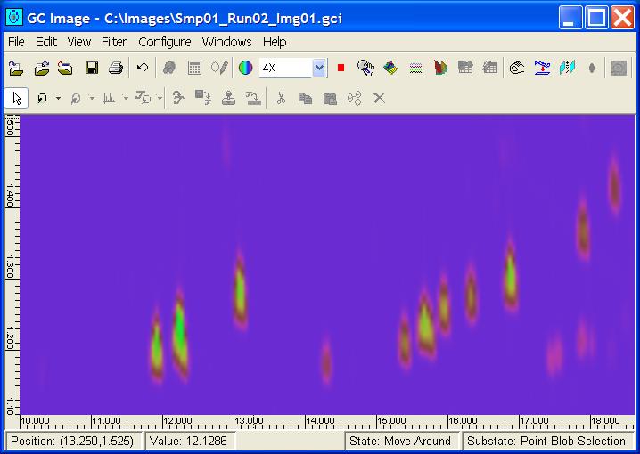
Figure 1: The Image Viewer with a region of a GCxGC image.
When an image is opened in GC Image, the Image Viewer is in
View cursor mode. To return to View mode from another
cursor mode, click the View mode button on the Image Viewer
palette.
In View cursor mode, it is possible to pan or scroll
about the image by click-and-drag with the left mouse-button.
For example, to slide the image to the left, depress the left
mouse-button (with the cursor in the Viewport), move the mouse
left, and release the left mouse-button. The arrow keys also can
be used for pan and scroll at increments of four pixels. The
page-up and page-down keys move a full screen up or down. (Note
that it is necessary to click in the Viewport to activate
the listeners for these keyboard actions.) There is also a special
navigation tool, the Navigator, described in the next section.
Change the magnification factor with the Scale Viewport control
on the Image Viewer tool bar or in the Navigator, described
in the next section.
To change the magnification in the Scale Viewport control, select
one of the values from the pull-down menu or enter the desired value
(followed by enter) in the text box.
The Viewport image is magnified using bi-linear interpolation.
Figure 1 pictures an open image with a sub-region displayed in the
Viewport at 4x magnification.
GC Image also supports more general resizing. Resize changes
the dimensions, including aspect ratio, used in display operations.
Resize operates on the full image buffer that is used in a
variety of operations. For example, resizing is useful before exporting
an image an external file format. Resize is different than the
scale operation in the Scale Viewport control and the
Navigator. The scale operation in Scale Viewport and
Navigator operates on the ROI in the Viewport and is
preferred for rescaled viewing.
Resize can be performed in View cursor mode by click-and-drag
of the right mouse-button in the Viewport. Then, the rectangular
region delimited is scaled and resized to fit the Viewport. (The
resize action is slightly more time consuming than scaling.) Successive
resize actions can be performed. The Display Reset button
resets the scale to 1 and the size to the original dimensions.
Resize also is available with a dialog interface accessible as
a choice on the View menu.
Navigator
The Image Viewer supports full resolution and magnified views
of the image, but only a sub-region of the image may be visible.
The Navigator provides a "thumbnail" view of the entire
image (typically at reduced resolution).
The Navigator also provides an interface to visualize and relocate
the region-of-interest (ROI) that is displayed in the Viewport
of the Image Viewer.
Figure 2 illustrates the Navigator.
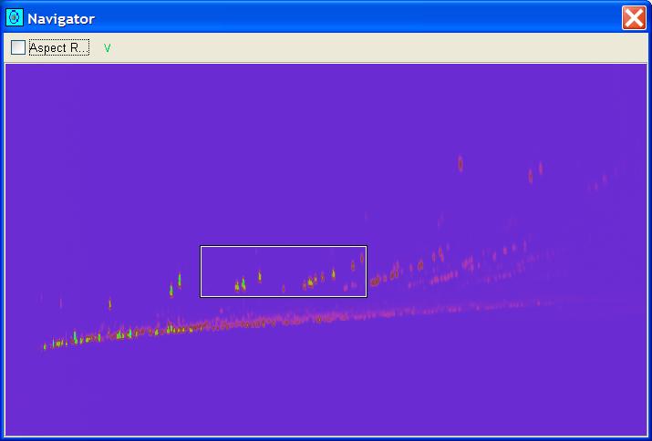
Figure 2: The Navigator with ROI specification
of the image in the Viewport.
Open the Navigator by clicking on the Navigator
button on the Image Viewer tool bar or by selecting
View->Navigator from the Image Viewer menu bar.
Close the Navigator by dismissing the window.
The graphic rectangular box in the Navigator is the region-of-interest
(ROI) that is displayed in the Viewport of the Image Viewer.
The ROI can be relocated by using the mouse to grab the box and drag
it to another location or via the Position Viewport button
on the Navigator tool bar.
The ROI can be resized by grabbing an edge or corner of the box and
dragging it.
When the ROI is relocated or resized, the image displayed in the
Viewport is changed accordingly.
Likewise, the ROI is relocated or resized when the Viewport is
moved or the Scale Viewport setting on the Image Viewer
tool bar is reset.
A popup from the Navigator allows precise specification of the
location for the ROI.
The size of the Navigator can be changed by grabbing
and dragging the border or corner of the window.
As the size is changed, the thumbnail image in the Navigator
is resized to fit the window, changing the magnification and/or aspect
ratio of the thumbnail image.
The user can indicate whether the aspect ratio in the Navigator
is maintained with a checkbox on the Navigator tool bar.
Colorize
GCxGC images have one double-precision value for each pixel.
A natural way of viewing images with one value per pixel is to use a
grayscale, in which values are displayed from black to white in various
shades of gray according to their magnitude, e.g., black for the
pixels with smallest value and white for the pixels with largest value
(or vice versa).
A grayscale provides a clear ordering of values from small to large.
Unfortunately, the human eye can distinguish only about 100 distinct
gradations on a grayscale, so the fabulous range of values present
in GCxGC images cannot be appreciated fully in grayscale.
Colorization allows the human eye to distinguish many more
distinct gradations in a GCxGC image.
Colorization uses three values to specify a color for each value in
the image.
Each pixel value is mapped through a color map to a corresponding
color, so two pixels with the same values will be displayed with the
same color and two pixels with different values may be displayed with
different colors.
With colorization, the ordering of values is not as straightforward
as with a grayscale, but a good color mapping scheme can provide a
clear progression. For example, topographic maps commonly use an
ordering from small to large that progresses through dark blue, light
blue, dark green, light green, light brown, dark brown, and red.
The GC Image Colorize tool allows user control over the color
mapping.
The Colorize tool supports:
-
Loading of pre-defined color maps.
-
Interactive specification and modification of color maps with:
-
either curve-fit or linear Color Map functions;
-
either Red-Green-Blue (RGB) or Hue-Saturation-Value (HSV) Color Model;
-
log-function Value Map; and
-
Color Wheel rotation.
-
Saving of user-defined color maps.
Open the Colorize by either clicking the Colorize button
on the Image Viewer tool bar or selecting View->Colorize
on the Image Viewer menu bar.
Figure 3 illustrates the Colorize window.
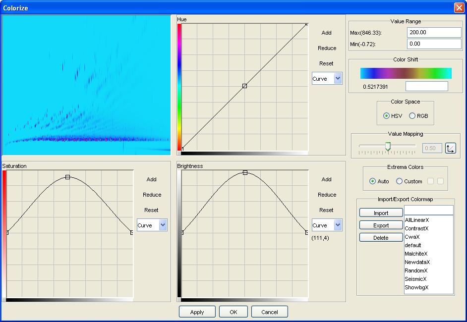
Figure 3: The GC Image Colorize tool.
The Colorize tool has several components:
-
A sub-region of the image from the ROI is displayed in the upper-left
corner of the Colorize tool.
The colorization changes can be previewed in this component.
-
Three Color Map functions, either RGB or HSV, depending on the current
color model, are displayed in the middle of the Colorize tool.
The Color Map horizontal axes are for the pixel value (after mapping
through the Value Map) over the current Value Range.
The Color Map vertical axes are the color component value (Red, Green,
or Blue for RGB or Hue, Saturation, or Value for HSV).
The Color Map functions assign color component values for each pixel
value in the Value Range.
The Color Map functions can be changed by grabbing and relocating
a knot, indicated with a small square.
As the cursor is moved in the graph, the cursor location is displayed
on the graph control panel.
The function is interpolated between the knots linearly or with a spline
curve and the interpolation method can be specified on the graph control
panel.
It is also possible to add and remove knots and to reset the function
(undoing changes made to the Color Map function).
-
When the Color Map functions are set as desired, they can be applied
to the image with the Apply button at the bottom of the
Colorize tool.
The OK button applies the current Color Map to the image and
dismisses the Colorize tool.
The Cancel dismisses the Colorize tool without applying the
Color Map.
-
The Value Range for color mapping is set at the top of the control
panel on the right side of the Colorize tool.
The Value Range is the range of values that are mapped (i.e.,
values between the Value Range minimum and maximum are color mapped).
Values outside the Value Range are set to the Extrema Colors
specified elsewhere on the control panel.
The labels on the minimum and maximum text boxes give the minimum and
maximum values in the image.
Note that after entering a desired minimum or maximum value, it is
necessary to enter the value by typing the ENTER or RETURN key on the
keyboard.
-
The three component color maps combine to form a color bar which can
be treated as a Color Wheel, with one end of the color scale
wrapped around to other end of the scale.
The Color Wheel can be rotated by click-and-drag on the color
bar or by specifying the shift (between 0 and 1).
The current shift is indicated in the shift textbox label.
Note that if the shift is changed by typing in the textbox, it is
necessary to enter the value by typing the ENTER or RETURN key on the
keyboard.
When using the Color Shift, the Extrema Colors (described
below) typically also should be set.
-
The Color Space is specified as either Hue-Saturation-Value (HSV)
or Red-Green-Blue (RGB) on the Colorize control panel below the
Color Shift.
-
The Value Map controls are below the Color Space controls.
A Value Map optionally remaps values as a log function of the value.
A Value Map setting equal to 0.5 is a linear mapping of the range
of pixel values to the color scale.
A Value Map setting less than 0.5 causes the color transitions to
be principally in the lower range of values and A Value Map setting
greater than 0.5 causes the color transitions to be principally in the
upper range of values.
The Value Map controls include a button to reset the mapping parameter
to 0.5 for linear mapping.
-
The color of pixels with values less than the minimum of the Value
Range or greater than the maximum of the Value Range can be
set as Extrema Colors.
The automatic setting is to use the color value of the Value Range
minimum value for all values less than the minimum and to use the
color value of the Value Range maximum value for all values greater
than the maximum.
The Extrema Colors controls, located below the Value Map
controls, also allow custom settings for these values.
-
The Import/Export controls allow users to access several color
maps supplied with GC Image and to save and load custom color maps.
These controls are located below the Extrema Colors controls at
the bottom of the Colorize control panel on the right side of the
Colorize tool.
To import a color map, select the desired map from the list of color
maps with a mouse click and then click the Import button.
To export a color map, enter the desired name for the color map in the
text box and then click the Export button.
To delete a color map, select the desired map from the list of color
maps with a mouse click and then click the Delete button.
The color map named default will be used whenever an image is
imported image without a color map.
Text View
The GC Image Text View tool provides a tabular view of the data
values, as illustrated in Figure 4.
Text View is available as a button on the Image Viewer
tool bar and as View->Text View from the Image Viewer
menu bar.
Terminate Text View by dismissing the window.
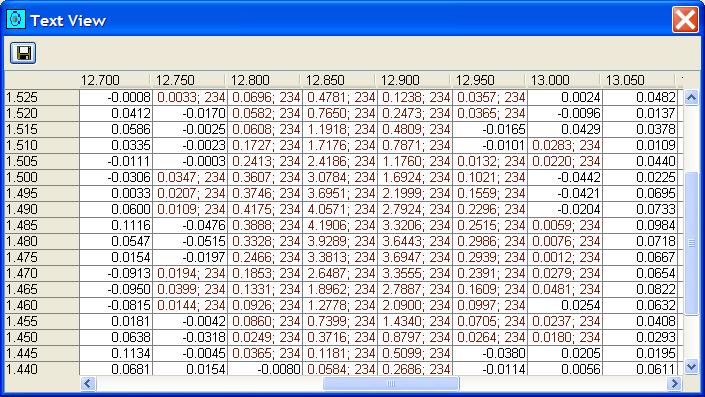
Figure 4: The GC Image Text View tool.
If a rectangular region is selected using the Graphics tool
(as described in chapter Graphics),
then only the values in the selected rectangular region are shown
in Text View.
If a single blob is selected, then only the values in the bounding box
of that blob are shown in Text View.
Otherwise, the entire image is available, which can entail extensive
scrolling.
If blobs have been detected for the image (as described in chapter
Detection and Analysis) then Text View
also reports the Blob ID at pixels that are a part of a blob and attempts
to highlight the blobs using distinct colors for the text in each blob.
Otherwise, if blobs have not been detected, the Text View shows
all values in black text.
The array of pixel values displayed in a Text View window can
be written to a text file in comma-separated-value (CSV) format.
Three-Dimensional Perspective View
The GC Image 3D View tool provides a three-dimensional perspective
view of the data values, as illustrated in Figure 5.
3D View is available as a button on the Image Viewer
tool bar and as View->3D View from the Image Viewer
menu bar.
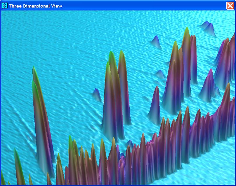
Figure 5: The GC Image 3D View tool.
The 3D View control panel, pictured if Figure 6, provides
scroll-bar control of viewing angle and distance, as well as controls
for wireframe or continuous surface, for monochromatic or colorized
surface, and for interpolation scaling. Configure->Configure
Settings also provides access to 3D View configuration
settings. Mouse actions also are supported: translate the image by
click-and-drag with the right mouse-button; rotate the image by
click-and-drag with the left mouse-button; and zoom (or scale) the
image by click-and-drag with the middle mouse-button.
Terminate 3D View by clicking the close button on the control
panel or by dismissing the 3D View window.
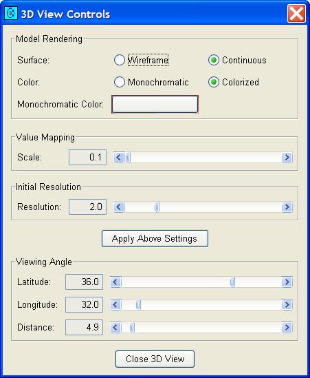
Figure 6: The 3D View control panel.
If a rectangular region is selected using the Graphics tool (as
described in chapter Graphics), then
only the selected rectangular region is shown in 3D View.
Otherwise, the entire image is available.
If blobs have been detected (and blob display is enabled), then
3D View will colorize the blob outlines.
Geometric operations in three-dimensional perspective viewing are
computationally intensive.
Future releases will implement additional features for three-dimensional
visualization.
Multi-Projections
The GC Image Multi-Projections tool supports graphing of
one-dimensional slices and projections of an image.
A projection is the one-dimensional sum across a range of rows or
a range of columns.
A slice is a single row or column (which is the projection with a
range of only one row or one column). The Multi-Projections
tool also supports multiple slices as described below.
Figure 7 illustrates the Multi-Projections window with graphs
of the selected row and column slices.
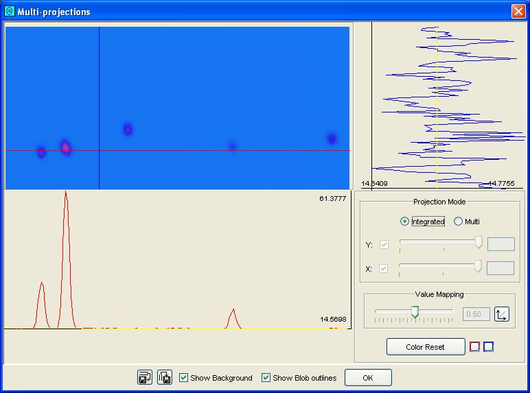
Figure 7: The GC Image Multi-Projections tool with
graphs of the selected row and column slices.
The Multi-Projections tool displays the sub-region of the image
from the ROI.
Clicking on a location in the sub-image in the Multi-Projections
tool specifies the row and column displays:
-
a one-dimensional graph of the pixel values from the specified row in
the panel below the image sub-region and
-
a one-dimensional graph of the pixel values from the specified column in
the panel to the right of the image sub-region.
The location of the sub-image can be moved left or right (or up or down)
by click-and-drag with the left mouse-button on the graph panels at the
bottom or left of the Multi-Projections tool.
The colors of each graph and associated column selector can be set
on the Multi-Projections tool control panel.
Optionally, the Multi-Projections tool will graph the estimated
baseline level for single slices.
Clicking and dragging in the sub-image display defines a range of
rows and columns.
With a range of rows and columns, there are two options:
-
Integrated projection: The pixel values from the selected rows
in each column are added together, yielding a vertical projection
graphed below the sub-image, and the pixel values from the selected
columns in each row are added together, yielding a horizontal projection
graphed to the right of the sub-image.
Figure 8 illustrates the integrated projection.
-
Multiple slices: The pixel values in several uniformly spaced
rows from the selected range of rows are graphed below the sub-image
and the pixel values in several uniformly spaced columns from the
selected range of columns are graphed to the right of the sub-image.
The Multi-Projections tool allows specification of the number
slices with the multiple slices option.
Figure 9 illustrates multiple slices.
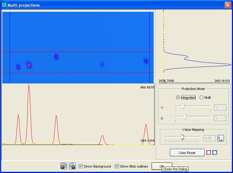
Figure 8: The GC Image Multi-Projections tool with
integrated projections from the selected rows and columns.
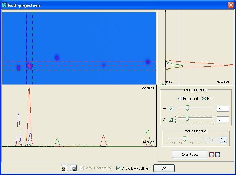
Figure 9: The GC Image Multi-Projections tool with
multiple slices from the selected rows and columns.
The slice, projection, or multi-slices along either the vertical or
horizontal dimension can be saved to a text file with buttons at the
bottom of the Multi-Projections tool.
Other checkboxes indicate whether or not baseline level is graphed
and blob outlines are displayed.
Visualize Data
GC Image supports visualization of various pixel statistics, as
illustrated in Figure 10.
If a rectangular region is selected using the Graphics tool (as
described in chapter Graphics), then
the statistics include only the pixels in the selected rectangular region.
Otherwise, the statistics include all pixels in the image.
The Visualize Data tool is launched from the Visualize
Data button on the Image Viewer tool bar or from
View->Visualize Data menu item.
Close Visualize Data by dismissing the window or clicking the
close button.
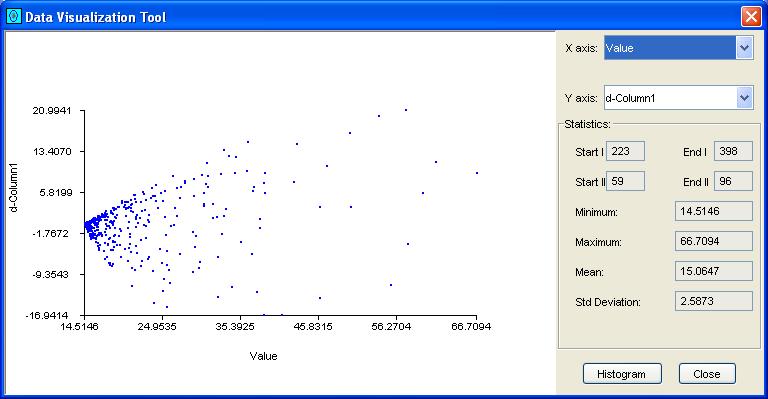
Figure 10: The GC Image Visualize Data tool.
Visualize Data reports several pixel statistics of the reported
rectangular region:
- the bounding box,
- the minimum and maximum pixel values, and
- the mean and standard deviation of pixel values.
Visualize Data contains a two-dimensional plot with
user-configurable values. The values that can be plotted are:
- pixel value,
- row and column indices, and
- discrete directional derivatives and gradient of value.
Visualize Data also offers a popup with a histogram plot
of pixel values, as pictured in Figure 11.
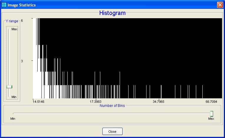
Figure 11: A histogram of pixel values.
The Visualize Data tool and the histogram popup are closed
with buttons or by dismissing the window.
Contents
Previous: Image Input and Output
Next: Graphics
GC Image™ Users' Guide © 2001–2004 by GC Image, LLC, and the University of Nebraska.