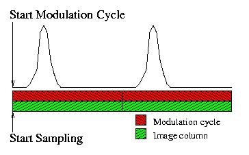
Figure 1.A: The start of sampling is synchronized with the start of the modulation cycle.
In GC Image, the Shift Phase operation is invoked by either
clicking the Shift Phase button on the Image Viewer tool
bar or selecting the Shift Phase item from the Filter menu.
The operation begins with a popup dialog box for entering the number
of pixels to be shifted. The shift can be a positive or negative number
for an upward or downward shift, respectively. The actual shift is set
to the number of pixels specified by the user modulo the number of pixels
in the second column separation.
The interface also supports resetting to the original phase.
Figure 2.A illustrates an image before Shift Phase.
The color scale is mapped over a narrow range to make the small blobs
at the top and bottom of the image more visible.
Note that some blobs wraparound to the bottom of the image.
Figure 2.B shows the image after Shift Phase of -75
pixels. The blobs that were wrapped around to the bottom of the image
are shifted back to the top of the image.
Figure 3 illustrates a perspective plot of an isolated peak rising
to a maximum value of over 23 pico-amps. However, the baseline in that
region of the image is more than 14 pico-amps, so the actual maximum
peak height induced by the sample chemical is less than 10 pico-amps.
In a simple model of the two-dimensional GC process, each image pixel
produced by the system is the sum of:
The GC Image Correct Baseline operation estimates the baseline across
the chromatographic image based on a few structural and statistical
properties of the two-dimensional chromatographic process.
Then, the baseline is subtracted from the image, producing a chromatograph
in which the peaks rise above a zero-mean baseline level.
(The noise is assumed to be zero-mean, in that any offset in the image
is modeled in the baseline.)
To perform the Correct Baseline operation, either click the
Correct Baseline button on the Image Viewer tool bar
or select the Correct Baseline item from the Filter menu.
The correction operation takes a brief time (typically no more
than a few seconds), after which the current image is altered.
After baseline correction, it may be desirable to re-colorize the
image to reflect the new range of values.
For details about this process, see "Background Removal and Peak Detection
in Two-Dimensional Gas Chromatography", Reichenbach, Ni, Zhang, and
Ledford, Journal of Chromatography A, 985(1-2):47-56, 2002.
Configure->Configure Settings on the Image Viewer menu bar
provides four parametric values for Baseline Correction:
Figure 4.A illustrates an image before baseline correction.
The image is for a blank run (i.e., no sample) and the
value range of the color map is set to be very small (13 picoamps
to 15 picoamps) in order to highlight the small but clear increase
in baseline value with time.
Figure 4.B illustrates the same image after Correct
Baseline (with a value range of -1 to 1).
The rise in the baseline level has been removed.
Note that baseline correction does not remove more quickly varying
acquisition artifacts.
Point-wise subtraction of a so-called blank run (a chromatographic
run with no sample input) can be used to remove background artifacts.
Point-wise addition of images can be used to obtain an average
chromatogram.
The first step in Mask Pixels is to select a rectangular or
polygonal region using the graphics tools (as described in the
chapter Graphics).
Then, to perform the Mask Pixels operation, either click
the Mask Pixels button on the Image Viewer tool bar
or select the Mask Pixels item from the Filter menu.
The Mask Pixels presents a popup interface in which the user
specifies the value of the pixels after masking and whether the pixels
interior or exterior to the selected region are masked.
Mask Pixels typically is performed after baseline correction
and with masked pixels set to value 0.
To remove an artifact, the typical operation is to outline the artifact
with a polygon and then set the pixels inside the polygon to 0.
To perform selective analysis, the typical operation is to outline the
desired region with a polygon and then set the pixels outside the
polygon to 0.
The correction operation takes a brief time, after which the current
image is altered.
In this version, GC Image does not support undoing of Mask Pixels.
The undo operation will be implemented in a later version.
Figure 6.A illustrates an image with a small horizontal stripe
of bleed that has been outlined with a polygon.
Figure 6.B illustrates the image after Mask Pixels, setting
pixels in the interior of the polygon to 0. The bleed stripe is eliminated.
The Detect Blobs operation produces a table of blob attributes or
features including peak location, area, volume, etc.
This structure can be viewed and edited with the tools described in
chapter Analysis.
The blob detection algorithm uses a greedy dilation that successively
attaches the largest-valued unassigned pixel to a neighboring blob or
forms its own blob if no neighboring peak has been established.
Configure->Configure Settings on the Image Viewer menu bar
provides parametric settings for Blob Detection:
Contents
Previous: Graphics
Next: Analysis
GC Image™ Users' Guide © 2003, 2002, 2001 by GC Image LLC and the University of Nebraska.

Figure 1.B: The start of sampling is not synchronized with
the start of the modulation cycle.

Figure 1.C: The image columns from the unsynchronized image
are brought back in alignment by padding the data.

Figure 2.A: An image before Shift Phase has wraparound.

Figure 2.B: An image after Shift Phase corrects wraparound.
Correct Baseline
In gas chromatography, the signal peaks, which correspond to chemical
constituents in the sample, rise above a baseline level in the output.
Under controlled conditions, the baseline level consists primarily of
the steady-state standing-current baseline in standard GC detectors and
temperature-induced column-bleed which causes a rise in the signal in
the later portions of temperature-programmed runs. Accurate
quantification of the chemical-related peaks requires subtraction of
the baseline level from the signal.

Figure 3: Perspective plot of a GCxGC sub-image containing an
isolated blob peak.
Under typical controlled conditions, the baseline offset values change
relatively slowly over time, forming a slightly curving baseline across
the image.
The signal and noise fluctuate more rapidly over time and so can be
separated from the slowly varying baseline offset.
The Filters menu also has an option to reset the image to its
original baseline offset (Undo Baseline Correction).
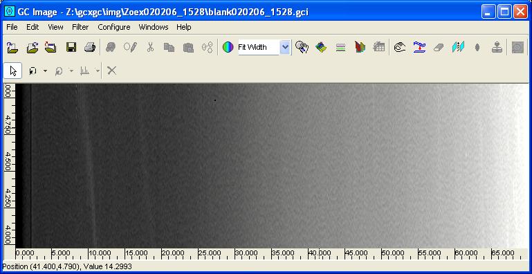
Figure 4.A: An image before Correct Baseline has a clear
increase in baseline level from left to right.

Figure 4.B: An image after Correct Baseline corrects
the baseline level.
Arithmetic Operations
GC Image provides for point-wise Arithmetic Operations, which
operate on a pixel-by-pixel basis. The currently supported operations
are addition, subtraction, and multiplication. The operands are the
current image and either a scalar value applied to all pixels or a GC
Image file specified by its filename. If a second image is specified,
it must have the same size in pixels as the current image. The
Arithmetic Operations popup is shown in Figure 5.

Figure 5: The Arithmetic Operations popup.
Mask Pixels
GC Image can set regions of pixels to a fixed value. This operation,
called Mask Pixels, is useful for a variety of purposes including
elimination of acquisition artifacts and selective analysis of data.
For example, ASTM 2887 is a standard method for estimating the boiling
range distribution of petroleum samples using gas chromatography. It
may be desirable to eliminate regions of the image containing only column
bleed and so more accurately determine the boiling range distribution
of the chemicals in the sample.
Similarly, it may be desirable to separately analyze alkanes and
aromatic hydrocarbons.
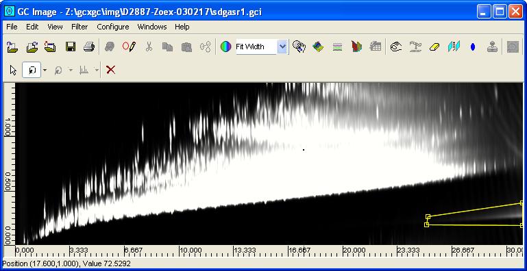
Figure 6.A: An image before Mask Pixels has a clear
acquisition artifact.
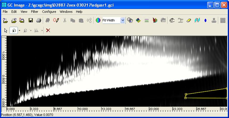
Figure 6.B: An image after Mask Pixels eliminates the
acquisition artifact.
Detect Blobs
GC Image can detect and quantify blob peaks in an image.
To perform the Detect Blobs operation, either click the
Detect Blobs button on the Image Viewer tool bar or
select the Detect Blobs item from the Filter menu.
The detection operation takes a brief time (typically no more
than a few seconds) and does not change the image.