Answers to questions about GC Image software.
- What is GC Image?
- How do I obtain GC Image software?
- How do I view GC Image version and license information?
- How do I view the GC Image Users' Guide?
GC Image is software for visualizing, processing, analyzing, and reporting on images produced in two-dimensional gas chromatography (GCxGC). GC Image was created by Dr. Stephen E. Reichenbach and others in the Computer Science and Engineering Department at the University of Nebraska - Lincoln and now is being developed by GC Image, LLC. For technical information about the GC Image software, contact
GC Image, LLCGC Image is proprietary software, with copyrights and trademarks held by GC Image, LLC, and the University of Nebraska - Lincoln.
PO Box 57403
Lincoln NE 68505-7403 USAPhone: 1.402.310.4503
Fax: 1.402.436.2660
Email: info@gcimage.com
For information about licensing the GC Image software, contact:
Zoex Corporation
Lincoln NE USAPhone: 1.402.475.7640
Email: info@zoex.com
Step 1: Select About GC Image from the Help menu of
the Image Viewer.

The About GC Image pop-up, with version and license information,
is displayed.

Step 1: Select Users' Guide from the Help menu of
the Image Viewer.

GC Image launches Microsoft Internet Explorer which displays the HTML-formatted GC Image Users' Guide.
Answers to questions about installing, starting, exiting, and uninstalling GC Image.
- What computer configuration is required for GC Image?
- How do I install GC Image software?
- How do I start GC Image?
- How do I set the license key in GC Image?
- How do I login to GC Image?
- How do add a user for GC Image?
- How do I retrieve a lost password?
- How do I exit GC Image?
- How do I uninstall GC Image?
GC Image software, Version 1.4 (February 2004), is distributed for installation on computer systems running a recent Microsoft Windows operating system, e.g., Windows NT (Service Pack 5 or later), Windows 2000, or Windows XP. The suggested minimum hardware configuration is a 1000MHz Intel Pentium 4 (or comparable) CPU, 512MB RAM (1024MB RAM is preferred, especially for GCxGC-MS), 32MB graphics card (64MB is preferred) and color monitor with 1024x768 (or higher) resolution. GC Image software requires relatively little hard-disk space (about 150MB), but images processed by the system (including the example images distributed with the software) may require large disk capacity.
Step 1: Execute setup.exe, a self-extracting program that installs the software. To install GC Image, the user must agree to the software license terms and conditions.
Step 2: Specify the folder location for the software.
The setup program adds a link to GC Image in the Start->Programs list and places a shortcut on the desktop.
Step 3: Follow the instructions for the NIST MS Search Demonstration software (if desired for GCxGC-MS data).
Step 4: Use the license number to obtain the license key from Zoex Corporation. Then, enter the license key in license popup.
Step 1: Execute GC Image from the Start->Programs, from the user-specified installation folder, or from the shortcut on the desk-top.
Note: This step is required only the first time the software is run after installation.
Step 1: Provide the license number to Zoex Corporation and get license key number.
Step 2: Enter the license key into the License dialog,
then click OK.

Step 1: Enter the username and password in the Login
dialog, then click OK.

Step 1: Click Add New User on the Login dialog.
Step 2: Enter the name, username, password (twice), and secret question and answer, then click OK.
Step 1: Click Forgot Password on the Login dialog.
Step 2: Enter the username on the Forgot Password dialog, then click OK to be shown the secret question.
Step 3: Enter the answer to the secret question and click Get Password. If the secret answer is correct, a popup will give the password.
Step 1: Select Exit from the File menu of the
Image Viewer.

When Exit is selected, the currently open image is discarded. If an image is open and has been altered since the Save or Save As operation for that image, GC Image prompts the user whether or not the image is to be saved before exiting. It is best to save changed images that are to be retained when they are changed to prevent the loss of unsaved work (e.g., in the event of a system crash or power failure) and before requesting the program to exit.
Step 1: Execute the uninstall program from the user-specified installation folder.
Answers to questions about input and output of GCxGC files in GC Image.
- What are the GCxGC file structures in GC Image?
- A file with .gci extension stores ancillary data about the image (e.g., its size, color mapping, etc.) in plain text format tagged using an eXtensible Markup Language (XML) schema for GCxGC images.
- A file with .bin extension stores the binary image data in time order with each value stored as an IEEE double-precision, floating-point number with big-endian byte order.
- What data formats can be imported by GC Image?
- How do I import GCxGC data?
- How do I open an image?
- How do I open a recently used image?
- How do I save an image?
- How do I save an image with a different file name?
- How do I export an image?
- How do I print an image?
- How do I close an image?
GC Image represents GCxGC images in two files:
GC Image can import images in a variety of file formats.
Extension Format .asc ASC - Thermo ASCII XY text format. Currently, metadata values are read for "Sampling Rate" and "Y Axis Multiplier". .bin Binary - big-endian, IEEE, single-precision, floating-point; optional byte-swapping supports little-endian format. .bmp Bitmap - common Microsoft Windows format. .cdf NetCDF - Analytical Data Interchange (ANDI) Protocol for Mass Spectrometric Data, based on the Unidata/UCAR network Common Data Format. Currently, not all ANDI metadata values are read. .ch CH - Agilent Chemstation IQ Data File Format. Currently, not all metadata values are read. .csv CSV - Comma-Separated-Values in text format; each line is "<time>, <value>" or each line has "<value>" only, without time or comma. .gif GIF - Graphics Interchange Format. .jpg JPEG - Joint Photographic Experts Group format. .png PNG - Portable Network Graphics format. .tif TIFF - Tagged Image File Format. .txt Text format; each line ends with a value, possibly preceded by other text separated by a tab, colon, semi-colon, comma, or space.
Step 1: Select Import Image from the File menu
of the Image Viewer (or the Import Image button from
the Image Viewer tool bar).
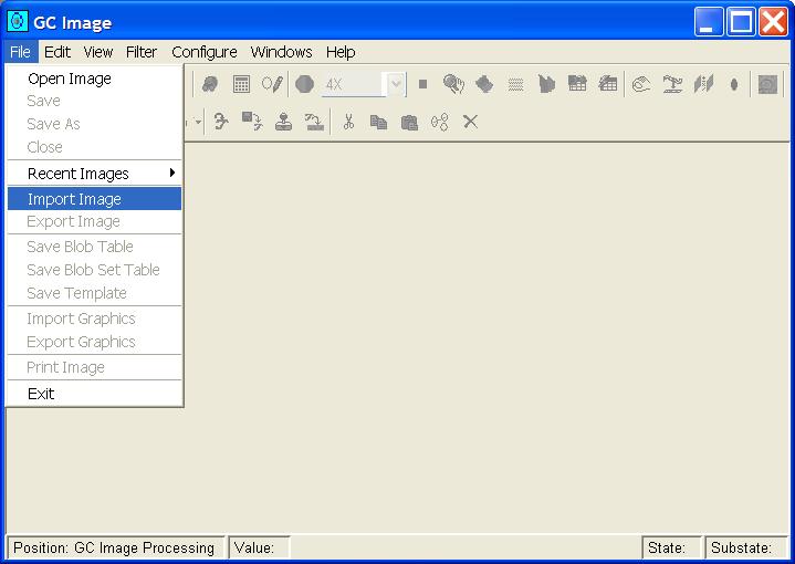
Step 2:
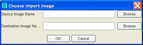
GC Image presents a pop-up dialog box for specifying the source and
destination folders and filenames.
Specify the source and destination folders and filenames,
either by typing in the text boxes or by using the file-system browsers.
The determination as to the input image file type is made on the basis of the file name extension, so files to be imported should be named with the proper extension. For more information on importing images, see chapter Image Input and Output.
Step 3: For file formats, such as CSV, that do not supply the
dimensions of the image, enter size parameters in the pop-up dialog
box for image dimensions.
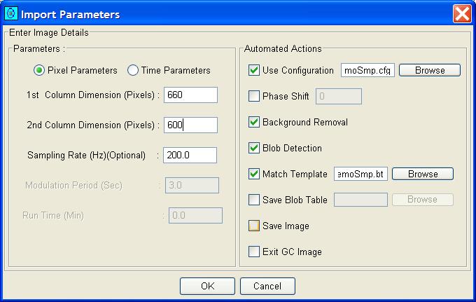
Step 4: If desired, choose to apply a specified processing configuration file and indicate the file.
Step 5: If desired, designate optional phase shift, optional background removal, optional blob detection (if background removal is performed), optional template matching with a specified template file (if blob detection is performed) with a specified template, optional saving of the blob table to a specified file (if blob detection is performed), optional saving of the image to a specified file, and optional exiting.
Step 1: Select Open Image from the File menu
of the Image Viewer (or the Open Image button from the
Image Viewer tool bar).

GC Image launches a file-system browser to locate the folder and
.gci file.

Step 2: Specify the folder and filename in the file-system browser.
Step 1: Select an image from the sub-menu list for the Recent
Images item on the File menu of the Image Viewer.

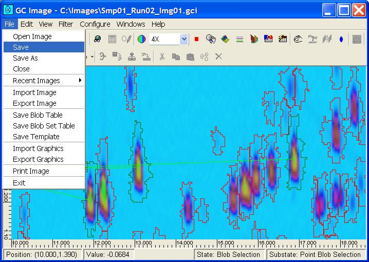
Step 1: Select Save from the File menu of the
Image Viewer (or the Save button from the Image Viewer
tool bar).
Step 1: Select Save As from the File menu of the
Image Viewer.

GC Image launches a file-system browser to specify the folder and
GCI .gci filename.

Step 2: Specify the folder and filename in the file-system browser.
Step 1: Select Export Image from the File menu
of the Image Viewer.

GC Image launches a file-system browser to specify the folder and
GCI .gci filename.

Step 2: Specify the folder and filename in the file-system browser. Also, choose to attach or not to attach axes to the exported image.
Step 1: Select Print Image from the File menu of the Image Viewer.
GC Image launches a print preview popup to specify the printing layout.

Step 2: Specify the printing layout and click the Print button.
Step 1: Select Close from the File menu of the
Image Viewer (or the Close button from the Image
Viewer tool bar).

When Close is selected, the current image is discarded. If the current image has been altered since the Save or Save As operation for that image, GC Image prompts the user whether or not the image is to be saved before closing. It is best to save all changed images that are to be retained when they are changed to prevent the loss of unsaved work (e.g., in the event of a system crash or power failure) and before requesting the image be closed. This menu option is not available if no image is open.
Answers to questions about viewing GCxGC images in GC Image.
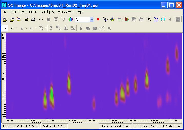
- What is the Image Viewer?
- title bar, which just displays the name of the current image;
- menu bar, which provides menu access to all operations, tools, settings, and help resources;
- tool bars, with buttons for commonly used operations, tools, and cursor modes;
- Viewport, which displays the region-of-interest of the current image with axes; and
- status bar, which displays the position and value of the image pixel at the cursor location.
- How do I resize the Image Viewer?
- How do I navigate (i.e., scroll and pan) about an image using the Image Viewer?
- How do I scale (or zoom) an image using the Image Viewer?
- How do I resize an image?
- How do I simultaneously scale and resize a region of interest?
- How do I reset the scale and size of the displayed image?
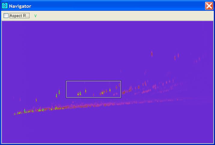
- What is the Navigator?
- How do I navigate (i.e., scroll and pan) about an image using the Navigator?
- How do I scale (or zoom) an image using the Navigator?
- How do I change the units on the Viewport axes?
The Image Viewer is the main interface of GC Image. The Image Viewer has (from top to bottom):
Step 1: With the cursor over a border or corner of the Image Viewer window, click-and-drag the border or corner to the desired size. (The Maximize button on the title bar makes the Image Viewer fill the screen and the Restore down button will restore the previous size after maximization.)
Step 1: Select View mode from the Image Viewer
cursor-mode palette.

Step 2: With the cursor in the Viewport, click-and-drag the image as desired. (Also, after clicking in the image, use the arrow, page-up, and page-down keys.)
Step 1: Select a value from the pull-down menu of scale factors
or type a value in the textbox in the Scale Viewport tool on the
Image Viewer tool bar.

Step 1: Select Resize from the View menu of the
Image Viewer.

GC Image launches a pop-up dialog box for the desired dimensions.

Step 2: Specify the desired values, then click OK.
Step 1: Select View mode from the Image Viewer cursor-mode palette.
Step 2: With the cursor in the Viewport, click-and-drag with the right-mouse button to delimit the desired region of interest.
Step 1: Click the Reset Display button on the Image Viewer tool bar.
The Navigator provides a "thumbnail" view of the entire
image (typically at reduced resolution).
The Navigator also provides an interface to visualize and relocate
the region-of-interest (ROI) that is displayed in the Viewport
of the Image Viewer.
The Navigator can be set to maintain aspect ratio or to fit the
image to the window.
Navigator can be launched by the too bar button or from the
View menu of the Image Viewer.
Step 1: With the cursor in the ROI box of the Navigator, click-and-drag the ROI to the position desired. More precise positioning can be specified via the Set Position button on the Navigator tool bar.
Step 1: With the cursor positioned on a corner of the ROI box of the Navigator, click-and-drag the corner of the ROI to the size desired.
Step 1: Select Configure Settings from the Configure
menu of the Image Viewer.

GC Image launches a pop-up with various configuration dialog panes.

Step 2: Select the Axes configuration pane.
Step 3: Select the desired units for the axes (e.g.., time or pixels). Click the OK button.
Answers to questions about colorizing GCxGC images in GC Image.
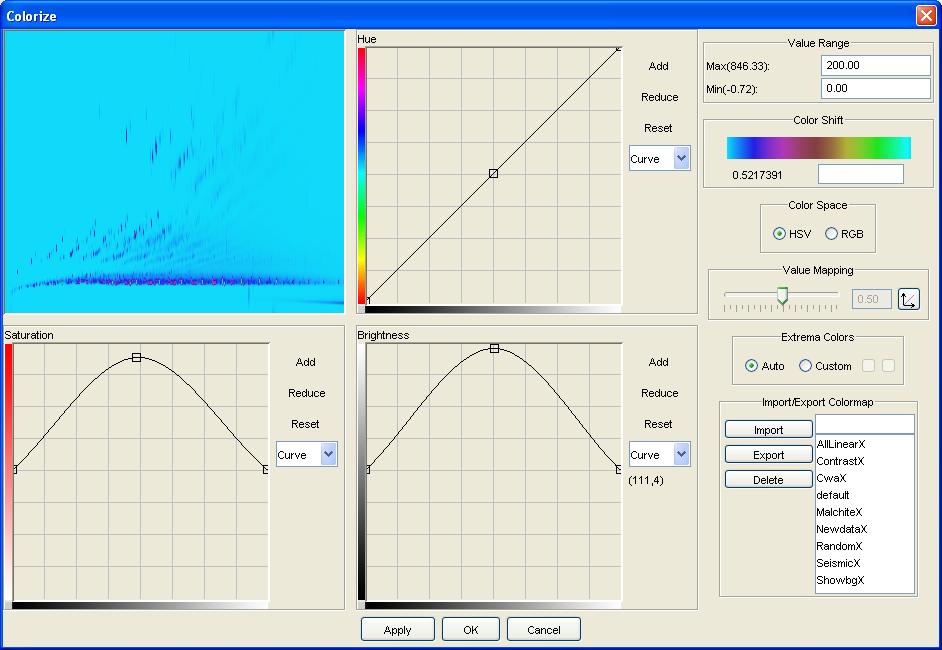
- What is colorization?
- How do I set the value range for colorization?
- How do I set the Extrema Colors for values outside the value range?
- How do I set Value Mapping for values within the value range?
- How do I set Color Mapping for values within the value range?
- How do I export Colorize settings?
- How do I import Colorize settings?
Colorization maps pixel values to colors for display. Within the user-configurable Value Range, values are mapped through a Value Map that applies a logarithmic, linear, or exponential function. Then, the value-mapped values are mapped through three Color Maps, using either Red, Green, and Blue (RGB) or Hue, Saturation, and Value (HSV or sometimes HSB for Brightness) Color Space. The Color Maps are defined using multiple knots and piecewise linear or cubic spline interpolation. The three color maps define a wheel that can be rotated with a Color Shift. Values outside the Value Range are set to Extrema Colors.
Open the Colorize tool by either clicking the Colorize button
on the Image Viewer tool bar or selecting View->Colorize on
the Image Viewer menu bar.
Step 1: Enter the minimum (Min) and/or maximum (Max) values
defining the value range in the text boxes in the upper-right corner
of Colorize. Type the ENTER or RETURN key on the keyboard to
enter the values.

Step 2: To apply the value range to the image, click the Apply button or the OK button.
Step 1: Select either automatically assigned (Auto) or user-specified
(Custom) Extrema Colors. (Automatically assigned Extrema Colors
are set to the colors of the minimum and maximum values.)

Step 2: For Custom Extrema Colors, click the left color box
to set the color for values less than the minimum and the right color box
to set the values greater than the maximum value. GC Image launches a
color chooser.

Step 3: In the color chooser, set the desired color using swatches, HSB sliders, or RGB sliders, then click the OK button.
Step 4: To apply the Extrema Colors to the image, click the Apply button or the OK button.
Step 1: Slide the Value Mapping slider left for logarithmic
value mapping or right for exponential value mapping or click the Value
Mapping button for linear value mapping.

Step 2: To apply the Value Mapping to the image, click the Apply button or the OK button.
Step 1: Select either RGB or HSV Color Space.

Step 2: Define the three color mapping functions by clicking to
add to or reduce the number of knots, click-and-drag the knots to the
desired positions, and choosing linear or spline interpolation through
the knots.

Step 3: To apply the Color Mapping to the image, click the Apply button or the OK button.
Step 1: Enter a name for the color map in the Import/Export
Colormap textbox.

Step 2: Click the Export button.
Step 1: Select a color map from the color map list.
Step 2: Click the Import button.
Answers to questions about image data visualization tools in GC Image.
- What image data visualization tools are available in GC Image?
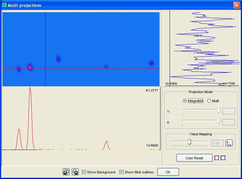
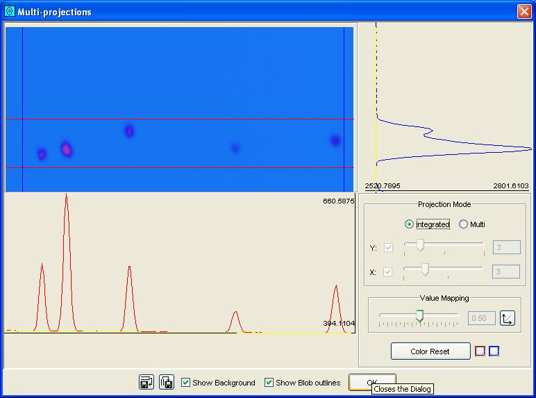
- Multi-Projections graphs one-dimensional slices and projections of an image.
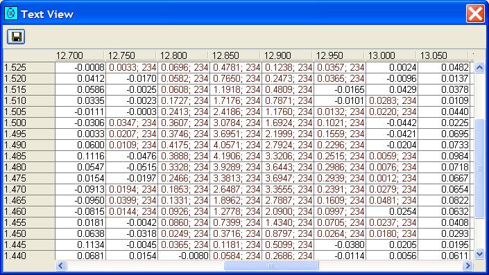
- Text View provides a tabular view of the image data values.
- 3D View tool provides a three-dimensional perspective view of the image data values.
- Visualize Data provides pixel statistics and plots statistical relationships for an image or sub-image.
- How do I view a one-dimensional slice of an image?
- How do I view a one-dimensional projection of an image?
- How do I view a multiple one-dimensional slices of an image?
- How do I save one-dimensional slices and projections of an image?
- How do I view the data values in a text table?
- How do I export the data values from a text table?
- How do I view the data values in a three-dimensional perspective view?
- Translate by click-and-drag with the right mouse-button.
- Rotate by click-and-drag with the left mouse-button.
- Zoom (or scale) by click-and-drag with the middle mouse-button.
- How do I configure the three-dimensional perspective view?
- How do I visualize pixel statistics?
GC Image provides several tools for visualizing image data.
Step 1: In the Multi-Projections control pane, select integrated projection mode.
Step 2: In the Multi-Projections image pane, click on a
pixel of the desired row and column. GC Image graphs the row slice at
the bottom of Multi-Projections and the column slice at the right
of Multi-Projections.
Step 1: In the Multi-Projections control pane, select integrated projection mode.
Step 2: In the Multi-Projections image pane, click-and-drag
from one side of the desired row and column range to the other side.
GC Image graphs the row projection at the bottom of Multi-Projections
and the column projection at the right of Multi-Projections.
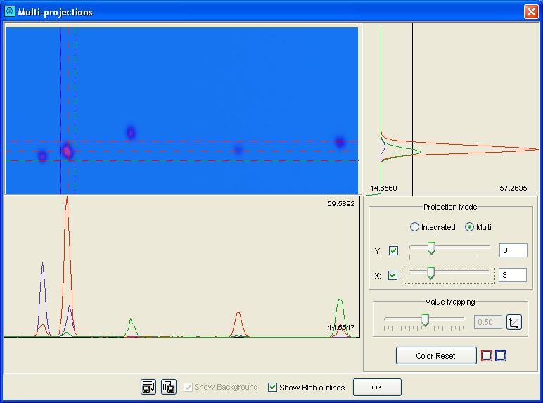
Step 1: In the Multi-Projections control pane, select multiple slices (Multi) projection mode.
Step 2: In the Multi-Projections image pane, click-and-drag from one side of the desired row and column range to the other side.
Step 3: In the Multi-Projections image pane, set the number
of horizontal and vertical slices with the sliders or enter values in the
text boxes and hit the RETURN or ENTER.
GC Image graphs the row slices at the bottom of Multi-Projections
and the column slices at the right of Multi-Projections.
Step 1: At the bottom of the Multi-Projections control pane, click either the horizontal or vertical save buttons. GC Image launches a file-system browser.
Step 2: Specify the file location and name for the CSV file.
Step 1: If desired, select a rectangular sub-region of the image, using the graphics tool for drawing rectangles, to see the values in the rectangle. Or, select a blob to see the values in the bounding box of the blob.
Step 2: Select Text View from the View menu of the
Image Viewer or click the Text View button on the Image
Viewer tool bar. GC Image launches a pop-up tool with the text table
of values.
Step 1: Click the Save text view button on the Text View popup. GC Image launches a file-system browser to specify the folder and CSV filename.
Step 2: Specify the file location and name, then click Save.
Step 1: If desired, select a rectangular sub-region of the image, using the graphic tool for drawing rectangles, to see the values in the rectangle.
Step 2: Select 3D View from the View menu of the
Image Viewer or click the 3D View button on the Image
Viewer tool bar. GC Image launches a pop-up tool with the three-dimensional
perspective view.
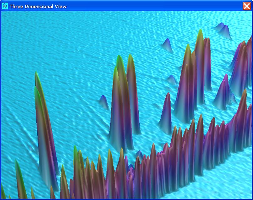
Step 3: Reposition the image using the latitude, longitude, and distance sliders on the 3D View control panel or with mouse actions:
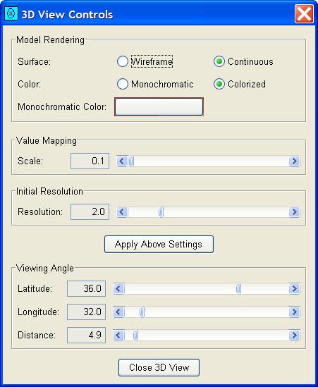
Step 1: On the 3D View control panel, select the surface as wireframe or continuous.
Step 2: Select the color as monochromatic or colorized. For a monochromatic display, select the color. For a colorized display, set the image color map.
Step 3: Select the initial resolution. Resolutions larger than 1.0 (the default) for large images may require more memory than is available and cause the program to fail.
Step 4: Click the Apply Above Settings button.
Step 1: If desired, select a rectangular sub-region of the image using the graphic tool for drawing rectangles.
Step 2: Select Visualize Data from the View menu
of the Image Viewer.
GC Image launches Visualize Data.
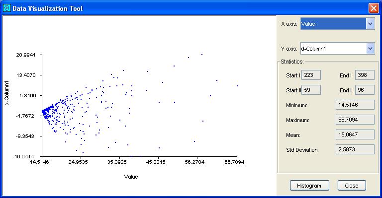
Step 3: Select the statistics for the X and Y axes.
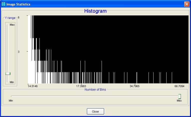
Step 4: If desired, click the Histogram button.
GC Image launches Histogram tool.
Answers to questions about graphics in GC Image.
- What graphics are available in GC Image?
- Select Graphic - Select a graphic.
- Draw Point - Draw a point.
- Draw Polyline - Draw a polyline.
- Draw Rectangle - Draw a rectangle.
- Draw Polygon - Draw a polygon.
- How do I draw and edit a point?
- How do I draw and edit a polyline?
- How do I draw and edit a rectangle?
- How do I draw and edit a polygon?
- How do I configure graphics display settings?
- How do I select a graphic?
- How do I select all graphics?
- How do I set and edit graphic(s) metadata?
- How do I delete a graphic?
- How do I export graphics?
- How do I import graphics?
GC Image supports point, polyline, rectangle, and polygon graphics. The Image Viewer palette contains a button to set the cursor mode to graphics and a pull-down graphics mode selector. The selectable graphic cursor modes are:

Step 1: Set the cursor mode to draw a point mode from the graphics cursor mode selector on the Image Viewer palette.
Step 2: Click at the desired location. After the click, GC Image
will revert to select a graphic mode with the drawn point selected.

Step 3: Click-and-drag on the point to move the graphic.
Step 1: Set the cursor mode to draw a polyline mode from the graphics cursor mode selector on the Image Viewer palette.
Step 2: Click the left mouse-button at each knot of the desired
polyline, except double click at the final knot to end the polyline.
After the polyline is ended, GC Image will revert to select a graphic
mode with the drawn polyline selected.

Step 3: Click-and-drag any knot handle(s) of the polyline to adjust points. Click-and-drag on the polyline to move the graphic.
Step 1: Set the cursor mode to draw a rectangle mode from the graphics cursor mode selector on the Image Viewer palette.
Step 2: Click-and-drag from one corner of the desired rectangle
to the opposite corner of the desired rectangle. After the mouse button
is released, GC Image will revert to select a graphic mode with the
drawn rectangle selected.

Step 3: Click-and-drag any corner handle(s) of the rectangle to adjust size. Click-and-drag from the interior of the rectangle to move the graphic.
Step 1: Set the cursor mode to draw a polygon mode from the graphics cursor mode selector on the Image Viewer palette.
Step 2: Click the left mouse-button at each vertex of the desired
polygon, except double click at the final vertex to close the polygon.
After the polygon is closed, GC Image will revert to select a graphic
mode with the drawn polygon selected.

Step 3: Click-and-drag any corner handle(s) of the polygon to adjust shape and size. Click-and-drag from the interior of the polygon to move the graphic.
Step 1: Select Configure Settings from the Configure menu of the Image Viewer. GC Image launches a pop-up with various configuration dialog panes.
Step 2: Select the Graphics Display configuration pane.

Step 3: Set whether to show graphics in all states or only in graphics cursor mode, set the color for drawing graphics, then click the OK button.
Step 1: Set the cursor mode to select a graphic mode from the
graphics cursor mode selector.
Step 2: Click on the existing graphic to be selected. Select additional graphics for the selection set by holding the control key during the click of the left mouse-button while the cursor is on the next graphic to be selected. GC Image will place handles on the selected graphic(s).
Step 1: Set the cursor mode to select a graphic mode from the graphics cursor mode selector.
Step 2: Select Select All item from the Edit menu. GC Image will select all graphics.
Step 1: Select one or more graphics using the select graphics cursor mode.
Step 2: Click the right mouse button. Depending on how many graphics
are selected, GC Image launches either a pop-up metadata dialog for a single
graphic or a pop-up metadata dialog for multiple graphics.


Step 3: For a single graphic metadata, set the desired name, description, inclusion flag, and color. For multiple graphics metadata, set the desired description, inclusion flag, and color.
Step 1: Select the existing graphic(s) to be deleted.
Step 2: Click the Delete / Exclude Object button.
Confirmation is required.

Step 1: Select Export Graphics from the File menu of the Image Viewer. GC Image presents a pop-up dialog box for specifying the destination file.
Step 2: Specify the destination file, then click Save.
Step 1: Select Export Graphics from the File menu of the Image Viewer.
Step 2: If graphics are present, GC Image prompts the user to overwrite or append to the existing graphics. Then, GC Image presents a pop-up dialog box for specifying the source file.
Step 2: Specify the source file, then click Open.
Answers to questions about image processing in GC Image.
- What image processing operations are available in GC Image?
- Shift Phase shifts the phase of the image with respect to the start time of the second dimension.
- Correct Baseline removes the slowly varying baseline (or background) level introduced by the system.
- Arithmetic Operations apply point-wise addition, subtraction, or multiplication with a scalar value or another image.
- How do I shift the second-column phase of an image?
- How do I reset shift of the second-column phase of an image?
- How do I correct the baseline offset of an image?
- How do I configure the baseline correction process?
- How do I perform point-wise arithmetic operations?
GC Image has three image processing operations.

Step 1: Select Shift Phase from the Filters menu
on the Image Viewer menu bar or click the Shift Phase
button on the Image Viewer tool bar.
GC Image launches a pop-up dialog box.

Step 2: Specify the desired phase shift (a positive value for upward shift and a negative value for downward shift) in the textbox, then click the OK button.
Step 1: Select Shift Phase from the Filters menu on the Image Viewer menu bar or click the Shift Phase button on the Image Viewer tool bar. GC Image launches a pop-up dialog box.
Step 2: Click the Reset button.
Step 1: Select Correct Baseline from the Filters menu on the Image Viewer menu bar or click the Correct Baseline button on the Image Viewer tool bar. GC Image applies the baseline correction algorithm, modifying the current image.
Step 1: Select Configure Settings from the Configure menu of the Image Viewer. GC Image launches a pop-up with various configuration dialog panes.
Step 2: Select the Baseline Correction configuration pane.

Step 3: Set the number of deadband pixels, filter window size, distribution, and stride parameters. Click the OK button. See chapter Image Processing for a description of the baseline correction algorithm and parameters.
Step 1: Select Arithmetic Operations from the Filters
menu in the Image Viewer.

Step 2: From the Arithmetic Operations popup dialog,
select the arithmetic operation, whether the operation is with
a scalar or image operand, and, for an image operand, the operand
file name. Then, click OK.

Answers to questions about blob detection in GC Image.
- What is blob detection?
- How do I detect blobs in an image?
- How do I configure blob detection?
- How do I configure blob display settings?
- How do I select blob(s)?
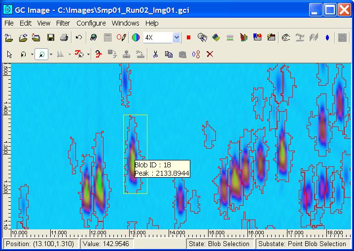
- In pixel blob-selection mode, move the cursor inside the border of a blob and click the left mouse-button. Select additional blobs for the selection set by holding the control key during the click of the left mouse-button while the cursor is inside the next blob to be selected.
- In line blob-selection mode, move the cursor to one side of a series of blobs, depress the left mouse-button, move the cursor to the other side of the series (defining a line through the series), and release the mouse button. All blobs crossed by the line will be selected.
- In rectangle blob-selection mode, move the cursor to a point above (or below) and left (or right) of all blobs to be selected, depress the left mouse-button, move the cursor below (or above) and right (or left) of all the blob peaks to be selected (defining a bounding box), and release the mouse button. All blobs with the peak pixel in the rectangle will be selected.
- In polygon blob-selection mode, move the cursor to a point near the blobs to be selected, click the left mouse-button, repeatedly move the cursor around the blobs to be selected and click the left mouse-button (drawing a polygon), and double click the left mouse-button (to close the polygon). All blobs with the peak pixel in the polygon will be selected.
- How do I select all blobs?
- How do I edit blobs with the Edit Blobs tool?
- How do I exclude blobs in the Image Viewer?
- How do I draw blobs in the Image Viewer?
Blob detection is the process of identifying the pixels that make up each peak. Once the blobs of pixels are detected, they can be visualized and analyzed. The position (i.e., the retention times in each dimension) of each blob is related to the physical properties the chemical that produced the blob, so the position of a blob is useful in identifying each chemical in a sample. The sum of the pixel values in each blob is related to the quantity of the chemical that produced it, so the sum of pixel values of a blob is useful in quantifying each chemical in a sample.
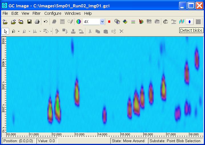
Step 1: Select Detect Blobs from the Filters
menu on the Image Viewer menu bar or click the Blob
Detection button on the Image Viewer tool bar.
GC Image detects the blobs and creates a blob table that can be
analyzed and reported.
The blobs are highlighted graphically in the Viewport of the
Image Viewer and in other tools according to blob display
configuration.
Step 1: Select Configure Settings from the Configure menu of the Image Viewer. GC Image launches a pop-up with various configuration dialog panes.
Step 2: Select the Blob Detection configuration pane.

Step 3: Set the number of detection algorithm, smoothing window, distribution, and filter parameters. Click the OK button. See chapter Image Processing for a description of the blob detection algorithm and parameters.
Step 1: Select Configure Settings from the Configure menu of the Image Viewer. GC Image launches a pop-up with various configuration dialog panes.
Step 2: Select the Blob Display configuration pane.

Step 3: Set what blobs to show, how to show blobs, whether to show internal standard associations, and colors. Click the OK button.
Step 1: Set the cursor mode to one of the blob selection
modes (point, line, rectangle, or polygon) from the graphics cursor
mode selector on the Image Viewers palette.
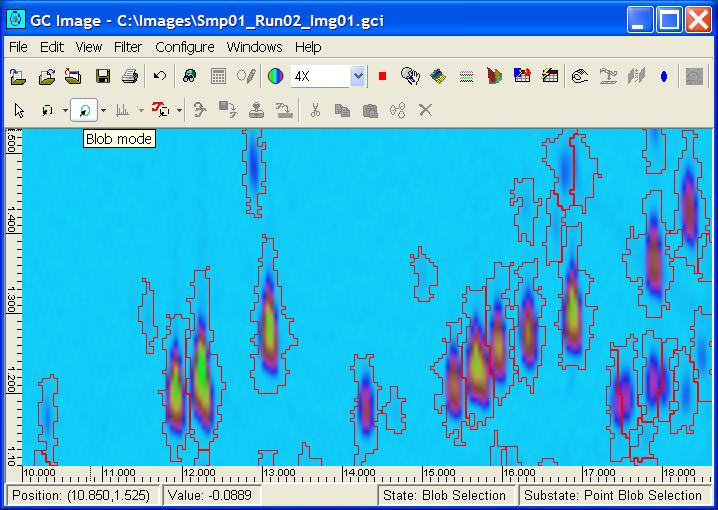
Step 2: Select blob(s) depending on the blob selection mode.
Step 1: Set the cursor mode to select blob mode.
Step 2: Select the Select All item from the Edit menu. GC Image will select all blobs.
Step 1: Select a focal blob using the blob selection cursor mode.
Step 2: Select Edit Blobs from the Edit menu on
the Image Viewer menu bar or the Edit Blobs button on
the Image Viewer tool bar.
GC Image launches Edit Blobs.

Step 3: Navigate the cross-hairs over the blob (or region) to be edited by click-and-drag in the image pane of Edit Blobs, Shift-Click in the image pane of Edit Blobs, or clicking the arrow navigation buttons.
Step 4: Use the operation buttons to split the blob vertically, split the blob horizontally, merge the blob with an adjacent blob, exclude the blob, or add a new blob.
Step 1: Select the blob(s) to be excluded.
Step 2: Click the Delete / Exclude Object button. Confirmation is required.
Step 1: Select the Draw Blob cursor mode.
Step 2: Click down on the mouse left-button, draw the cursor around the border of the blob (without crossing the line drawn or other blobs), and release the button to close the shape.
Answers to questions about blob statistics and metadata in GC Image.
- What blob statistics and metadata are available in GC Image?
- peak indices - the indices of the largest valued sample in the blob,
- peak value - the largest value in the blob,
- area - the number of pixels in the blob, and
- volume - the sum of pixel values in the blob.
- compound name - the name of the chemical compound associated with the blob,
- group name - the name of a chemical group to which the chemical compound associated with the blob belongs,
- inclusion flag - whether the blob is identified for inclusion in reporting,
- exclusion flag - whether the blob is identified for exclusion from all computations in reporting,
- internal standard - whether the chemical compound associated with the blob is an internal standard.
- How do I set and edit metadata for blob(s)?
- How do I cut, copy, and paste metadata for blob(s)?
- How do I view the blob table?
- How do I select blobs from the blob table?
- How do I save the blob table?
- How do I configure the blob table?
- Include desired feature(s) by click-and-pointing invisible feature(s), using Shift-Click to select a range and control-click to select additional features, and then clicking the add button.
- Un-include feature(s) by click-and-pointing visible feature(s) and then clicking the remove button.
- The feature list can be ordered by selecting the location for changed features on the destination list.
- How do I create a blob set?
- How do I view the blob set table?
- How do I select blobs from the blob set table?
- How do I save the blob set table?
- How do I find/select blobs by blob ID, compound name, group name, or constellation name?
- How do I perform quantitative selection or deselection of blobs?
- How do I visualize blob statistics?
- How do I use blob statistics visualizations for analysis?
GC Image supports more than 80 statistical features and metadata for blobs. See the white paper, GCxGC Blob Metadata and Statistics in GC Image, for details of each of the available metadata and computed attributes in GC Image. A few basic of the statistical features computed by GC Image are:
Step 1: Select one or more blobs using the select blobs cursor mode.
Step 2: Click the right mouse button. Depending on how many blobs
are selected, GC Image launches either a pop-up metadata dialog for a single
blob or a pop-up metadata dialog for multiple blobs.
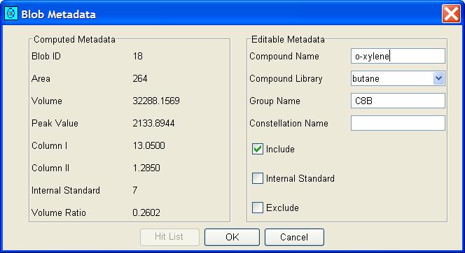

Step 3: For a single blob metadata, set the desired compound name, group name, constellation name, inclusion flag, internal standard flag, and exclusion flag. For multiple blobs metadata, set the desired group name, constellation name, inclusion flag, internal standard flag, and exclusion flag.
Step 1: Select a blob(s) using the blob selection cursor. (Metadata Cut will work for multiple blobs, but Copy Metadata and Paste Metadata will not for multiple blobs.)
Step 2: Select Cut Metadata, Copy Metadata, or Paste Metadata from the Edit menu of the Image Viewer or click the appropriate button on the Image Viewer bar. GC Image modifies the blob table accordingly.
Step 1: Select Blob Table from the View menu
of the Image Viewer or click the Blob Table button
on the Image Viewer tool bar.
GC Image launches Blob Table viewer.
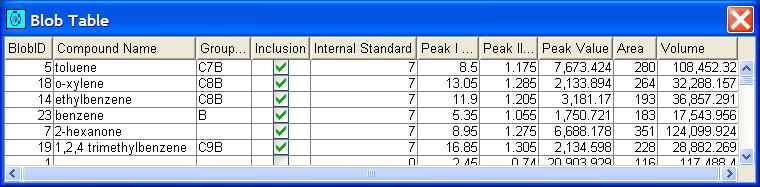
Step 2: Use the scroll bars to navigate the blob table. Sort the table by clicking on a column header (and click again to reverse order).
Step 1: Bring up the blob table.
Step 2: Click on a row of the blob table selects the blob. Click and click again with the shift key selects a range of blobs. Click with the control key adds a selection. Selected blobs are highlighted graphically in the Image Viewer.
Step 1: Select Save Blob Table from the File menu
of the Image Viewer.
GC Image launches a pop-up dialog.

Step 2: Enter the file name for the CSV .csv file, using
the file-system browser if desired, and indicate whether all blobs or
only included blobs are written to the file.

Step 1: Select Configure Blob Table from the Configure
menu of the Image Viewer.

GC Image launches the Configure Blob Table pop-up dialog.

Step 2: Select the desired features.
Step 1: Create a graphic object.
Step 2: Set the inclusion flag for the graphic object. For point and polyline graphics, the blob set is defined by intersection of the graphic with blobs. For a rectangle and polygon graphics, the blob set is defined by containment of the blob peaks by the graphic.
Step 1: Select Blob Set Table from the View menu
of the Image Viewer or click the Blob Set Table button
on the Image Viewer tool bar.
GC Image launches the Blob Set Table viewer.

Step 2: Use the scroll bars to navigate the blob set table. Sort the table by clicking on a column header (and click again to reverse order).
Step 1: Bring up the blob set table.
Step 2: Click on a row of the blob set table selects the blobs in the blob set. Click and click again with the shift key selects a range of blobs. Click with the control key adds a selection. Selected blobs are highlighted graphically in the Image Viewer.
Step 1: Select Save Blob Set Table from the File
menu of the Image Viewer. GC Image launches a pop-up dialog.

Step 2: Enter the file name for the CSV .csv file, using
the file-system browser if desired.

Step 1: Select Find Blobs from the Edit menu of the
Image Viewer.
GC Image launches a pop-up dialog.

Step 2: Select the desired criteria. Then click the OK button.
Step 1: Select Filter Blobs from the Filter menu
of the Image Viewer.
GC Image launches a pop-up dialog.

Step 2: Select the desired area, volume, peak value, and volume ratio values to filter blobs, then indicate filtering for selection or deselection.
Step 1: Optionally, select one or more blobs. (Otherwise, all blobs are visualized.)
Step 2: Select Visualize Blobs from the View menu
of the Image Viewer.
GC Image launches a tool for graphing bi-variate relationships for blob
statistics.

Step 3: Select the desired blob statistic for each axis.
Step 1: Perform Visualize Blobs.
Step 2: Designate a set of points in the graph by drawing a polygon
around them - clicking at each vertex and double-clicking at the final
vertex.

Step 3: Click the Assign Properties button to bring up a popup for setting the selected blobs metadata.
Step 4: Set the properties of the designated blobs and click the OK button.
Answers to questions about pattern recognition in GC Image.
- What are templates?
- Select template object - Select a graphic.
- Draw template point - Draw a template point.
- Draw template polyline - Draw a template polyline.
- Draw template rectangle - Draw a template rectangle.
- Draw template polygon - Draw a template polygon.
- Draw template peak - Draw a template peak (as a point).
- How do I add selected blob peaks to a template?
- How do I add selected graphics to a template?
- How do I draw and edit peaks and graphic objects in a template?
- How do I configure template display settings?
- How do I select template object(s)?
- How do I select all template objects?
- How do I set and edit template object(s) metadata?
- How do I delete template object(s)?
- How do I save a template?
- How do I load a template?
- How do I match a template to blobs in the image?
- How do I apply a matched template to blobs in the image?
- How do I configure template matching?
Templates are patterns of peaks and graphic objects observed in previous image(s) used to recognize similar patterns of blobs in subsequent image(s). Once recognized, the metadata (including chemical name, group name, and internal standard association) for the blobs in the target image can be set from the template. GC Image has tools for creating and using templates. The selectable template cursor modes are:

Step 1: Select blob(s), with metadata set as desired, to be included in the template.
Step 2: Click the Add to template button.

Step 1: Select graphic(s), with metadata set as desired, to be included in the template.
Step 2: Click the Add to template button.
Step 1: Set the cursor mode to the desired draw template object mode (point, polyline, rectangle, polygon, or peak) from the template cursor mode selector on the Image Viewer palette.
Step 2: Draw the desired template object using the same operations as for graphic objects. (Template peaks are drawn at designated locations, just as points are drawn.) After drawing, GC Image will revert to select a template object mode with the drawn template object selected.
Step 3: Edit the position and shape of the template object using the same operations as for graphic objects.
Step 1: Select Configure Settings from the Configure menu of the Image Viewer. GC Image launches a pop-up with various configuration dialog panes.
Step 2: Select the Template Display configuration pane.

Step 3: Set the color for the various classes of objects (included, unflagged, excluded, internal standards, and internal standard association lines) and the visibility for internal standard association lines, then click the OK button.
Step 1: Set the cursor mode to select a template object mode
from the template cursor mode selector.
Step 2: Click on the existing template object to be selected. Select additional template objects for the selection set by holding the control key during the click of the left mouse-button while the cursor is on the next template object to be selected. GC Image will place handles on the selected template objects(s).
Step 1: Set the cursor mode to select a template object mode from the template cursor mode selector.
Step 2: Select Select All item from the Edit menu. GC Image will select all template objects.
Step 1: Select one or more template peaks or one or more template graphics using the select template object cursor mode. (Metadata for template peaks and template graphics cannot be edited together.)
Step 2: Click the right mouse button. Depending on how many
template peaks or template graphics are selected, GC Image launches
either a pop-up metadata dialog for a single object or a pop-up metadata
dialog for multiple objects. The metata dialogs for template graphic
objects are the same as for graphic objects. The metadata dialogs for
template peaks are shown below.


Step 3: Enter the metadata settings, then click OK.
Step 1: Select the existing template object(s) to be deleted.
Step 2: Click the Delete / Exclude Object button. Confirmation is required.
Step 1: Select Save Template from the File menu of
the Image Viewer.
GC Image launches a file-system brower to specify the destination file.

Step 2: Specify the destination filename, then click the Save button.
Step 1: Select the Load Template option from the
Filter menu or click the Load Template button.
GC Image presents a dialog that allows the user to browse template
files with a graphical overlay on the image before loading (i.e.,
without modifying the image template).

Step 2: Browse and select the desired template, specify whether the existing template is to be overwritten or appended, then click Load. Template peaks and graphics must be unique, so any conflicting objects will not be appended and a message will be displayed in a popup.
Step 1: Perform blob detection and create or load a template.
Step 2: Select Match Template from the File menu
of the Image Viewer or click the Match Template button on
the Image Viewer tool bar. GC Image graphically highlights
peak-to-blob matches. Template peak matches are shown as color-filled
circles at the matched location. If not all peaks are matched, a popup
reports the matching failures. Note that Match Template does
not change the image or the template, it merely graphically visualizes
the matches.

Step 1: Perform Match Template.
Step 2: Select Apply Template from the File menu of the Image Viewer or click the Apply Template button on the Image Viewer tool bar.

Step 1: Select Configure Settings from the Configure menu of the Image Viewer. GC Image launches a pop-up with various configuration dialog panes.
Step 2: Select the Template Matching configuration pane.
Step 3: Set the search window for translation and scale of the template and the maximum distance (i.e., threshold) for matching between a template peak and blob peak. Click the OK button.
Answers to questions about configuration files and operations journals.
- What is a configuration file?
- How do I export (i.e., save) a configuration file?
- How do I import (i.e., load) a configuration file?
- What is an operations journal?
- View the list of operations.
- Undo the most recent operation.
- Report the journal.
- How do I view the list of operations that have been performed on an image?
- How do I undo the most recent operation performed on an image?
- How do I generate a formatted report of the operations journal?
GC Image provides a means of storing and recalling all the many configuration settings for processing and analyzing images, the color map, and the blob table configuration in a processing configuration file.
Step 1: Choose Configure Settings from the Configure menu of the Image Viewer. This presents a configuration pane.
Step 2: Click the Export Configuration button on any of
the configuration panes. This presents a popup dialog.

Step 3: Select the filename and indicate whether the blob table configuration and/or the color map are to be included.
Step 1: Choose Configure Settings from the Configure menu of the Image Viewer. This presents a configuration pane.
Step 2: Click the Import Configuration button on any of the configuration panes. This presents a file system browser to select a configuration file.
Step 3: Select the configuration file to be imported (i.e., loaded).
An operations journal is a record of the operations that have been performed on an image. Each entry in the journal includes the name of the operation, the parameters that were used in applying the operation, and all information that is required to undo the operation. The operations journal supports three operations:
Step 1: Select the List Operations option from the
Edit menu of the Image Viewer. GC Image presents a
popup with a text box listing a brief description for each operation
that has been performed on the image.

Step 2: Close the List Operations popup by clicking the OK button.
Step 1: Click the Undo button or select the Undo option from the Edit menu of the Image Viewer. The last operation that was performed to modify the image will be reversed.
Step 1: Select the List Operations option from the Edit menu of the Image Viewer. GC Image presents a List Operations popup.
Step 2: Click the View Journal button on the List Operations popup. The user is prompted to name the destination file for the report.
Step 3: Enter the destination file name for the report, then
click Save.

Answers to questions about GCxGC-MS data in GC Image.
- What GCxGC-MS tools are available in GC Image?
- input and output;
- viewing mass spectra of samples, peaks, and blobs;
- selecting mass/z subranges of mass spectra;
- generating ion chromatograms;
- constructing and applying selection expressions;
- searching mass spectral libraries; and
- using mass spectral library searches for blob identification;
- What are the file structures for GCxGC-MS data?
- a GCI file containing metadata (as described in chapter Image Input and Output) and
- a binary file containing the data in the Network Common Data Format (NetCDF).
- How do I import GCxGC-MS data?
- How do I perform input and output of GCxGC-MS data?
- How do I view a mass spectrum at a point?
- How do I view a mass spectrum at a blob peak?
- How do I view a mass spectrum for a blob?
- How do I select mass/z subranges of a mass spectrum?
- How do I generate an ion chromatogram image?
- How do I configure mass spectral and ion chromatogram display?
- How do I construct and apply selection expressions?
- How do I search a mass spectral library?
- How do I configure mass spectral searching?
- How do I use mass spectral library searches for blob identification?
- How do I correct blob mis-identifications made by mass spectral library search?
GC Image provides GCxGC-MS tools for:
GC Image stores GCxGC-MS data in two files:
GC Image supports importing GCxGC-MS data from files in CDF. To import GCxGC-MS data contained in a CDF file. Follow the same steps as for importing GCxGC data.
Using the GCI and CDF files, the GC Image file operations Open, Recent Images, Save, Save As, Close, and Exit work for GCxGC-MS images as they do for GCxGC images (chapter Image Input and Output).
Step 1: Select Point Mass Spectrum mode on the Image
Viewer palette.

Step 2: Click on a point in the total ion count (TIC) image.
Step 1: Perform blob detection.
Step 2: Select Peak Mass Spectrum mode on the Image Viewer palette.
Step 3: Click within a blob in the total ion count (TIC) image.
Step 1: Perform blob detection.
Step 2: Select Blob Mass Spectrum mode on the Image Viewer palette.
Step 3: Click within a blob in the total ion count (TIC) image.
Step 1: Display a point, peak, or blob mass spectrum.
Step 2: Within the graph area of the Mass Spectrum Viewer, click-and-drag the left mouse-button to designate the desired subrange.
Step 3: If desired, change the subrange by repeating Step 2 or
add additional subranges by repeating Step 2 with the control key
depressed.

Step 1: Select a mass/z subrange.
Step 2: Click the Ion Chromatogram button on the
Mass Spectrum Viewer.

Step 1: Select Configure Settings from the Configure menu of the Image Viewer. GC Image launches a pop-up with various configuration dialog panes.
Step 2: Select the Multi-Channel configuration pane.
Step 3: Select display for mass spectra in a single window or
multiple windows and display for spectal images in a single window or
multiple windows.

Step 1: Click the Select Expression button or choose the
Select Expression item from the View menu. GC Image presents
the Selection Tool.

Step 2: Build or load a selection expression.
Step 3: Click Select Blobs to select blobs satisfying the expression or click Generate Selection Image to generate an image masked to reveal only pixels satisfying the expression.
Step 1: Display a point, peak, or blob mass spectrum. If desired, select one or more mass/z subranges.
Step 2: Click the Search MS Library button on the Mass Spectrum Viewer.
Step 1: Select Configure Settings from the Configure menu of the Image Viewer. GC Image launches a pop-up with various configuration dialog panes.
Step 2: Select the Search MS Library configuration pane.

Step 1: Perform blob detection.
Step 2: Click the Search MS Library button on the Image Viewer tool bar or select Search MS Library from the Filter menu.
Step 1: Select the mis-identified blob using the select blobs cursor mode.
Step 2: Click the right mouse button. GC Image launches a pop-up
metadata dialog for a single blob.

Step 3: Click the Hit List button. GC Image launches a
hit-list popup.

Step 4: Click Select flag for the correct chemical identification, then click OK.
Questions about project management and reporting in GC Project.
- What tools are available in GC Project for project management and reporting?
- What is a project?
- Vials for composition files,
- Runs for raw chromatographic data,
- Processing for processing files,
- Images for processed image files, and
- Reports for report files.
- What is a vial in a project?
- What is a run in a project?
- What is a processing file in a project?
- What is a processed image in a project?
- What is a batch in a project?
- What is a report in a project?
GC Project provides support for organizing and reporting on the sets of data developed during GCxGC analyses. GC Project is invoked from the desktop icon, from the Microsoft Windows Programs menu, or from the installation directory.
The GC Project graphical user-interface (GUI) has a title bar, menu bar, tool bar, project tree, and component information pane. The lower-left pane contains the Project Tree that visualizes and provides access to the project components. The lower-right pane presents Component Information about the user-selected component(s) and provides access to component operations.
A node in the project tree can be selected by clicking on it. This
causes information about the node and buttons for relevant operations
to be displayed in the Component Information pane. Some nodes
(e.g., image nodes) have actions initiated by double-clicking
(e.g., opening the image with GC Image).
In the Project Tree, if a node has a '+', then it can be expanded
by clicking the '+' to list the children in the tree. If a node has a '-',
then it can be collapsed by clicking the '-' so that the list of children
is not shown. If there is neither a '+' nor '-', then there are no
children of the node.

A project consists of a directory named for the project, a GC Project file named for the project with extension .gcp in the project directory, and sub-directories:
Vials are elements that describe the different mixtures analyzed in the project.
Runs are unprocessed chromatograms.
Processing files are files used for processing chromatograms into images, including configuration files, blob templates, and graphics files.
Processed images are the results of processing and analyzing raw chromatograms using GC Image.
Batches are sets of processed images that are conveniently grouped for reporting.
A report is a formal presentation of information about processed images. Reports are formatted as XML (preferred), HTML, or CSV.
Questions about project files and directories in GC Project.
- How do I start GC Project?
- How do I create a new project?
- How do I save a project?
- How do I open an existing project?
- How do I close a project?
- How do I exit GC Project?
- How do I import composition tables into a project?
- How do I import raw chromatographic data into a project?
- How do I import processing files into a project?
Step 1: Execute the GC Project desktop icon, or choose GC Project from the Microsoft Windows Programs menu, or execute GC Project from the installation directory.
Step 1: Click the New Project button on the tool bar or select New Project from the File menu of GC Project.
Step 2: Specify the directory location and the project name.
Step 1: Click the Save Project button on the tool bar or select Save Project from the File menu of GC Project.
Step 1: Click the Open Project button on the tool bar or select Open Project from the File menu of GC Project.
Step 2: Specify the GC Project (extension .gcp) file in the file browser.
Step 1: Click the Close Project button on the tool bar or select Close Project from the File menu of GC Project.
Step 2: If the project has been modified since the most recent save operation, indicate whether or not the project should be saved.
Step 1: Select Exit from the File menu of GC Project.
Step 1: Create or copy a CSV file containing the composition table for each vial into the Vials subdirectory (under the project directory). The format is text with each line "<compound-name>,<amount>". Compound names containing commas should be enclosed in double quotation marks.
Step 1: Copy raw chromatogram files (e.g., CSV format) for each run into the Runs subdirectory (under the project directory). The file format must be readable by GC Image.
Step 1: Copy GC Image processing files (e.g., configuration files, blob templates, and graphics files) into the Processing subdirectory (under the project directory).
Questions about vials in GC Project.
- How do I view the list of vials in a project?
- How do I create vials in a project?
- How do I view information about a vial in a project?
- How do I import a composition table for a vial?
- How do I add a record to a composition table for a vial?
Step 1: Click the Vials node in the Project Tree.
Step 1: Click the Vials node in the Project Tree.
Step 2: Click the Add Vial button in the Component
Information pane.

Step 3: Specify the root-name of the vial, a starting sequence number for the vial, the number of vials to be created (with the sequence number incremented for each new vial), and vial metadata. Click the OK button.
Step 4: If there is a CSV-format composition table in the Vials directory with the same name as the vial, confirm or deny importation of the table.
Step 1: Expand the Vials node in the Project Tree.
Step 2: Select a Vial node in the Project Tree.

Step 1: View a vial in the Component Information pane.
Step 2: Click the Import Composition button.
Step 3: Specify the composition file (CSV format) in the file browser.
Step 1: View a vial in the Component Information pane.
Step 2: Click the Add Record button.

Step 3: Enter the compound name and amount, then click the OK button.
Questions about runs in GC Project.
- How do I view the list of runs in a project?
- How do I associate raw chromatographic data in a project?
- How do I unassociate a run in a project?
- How do I view information about a run in a project?
- How do I initiate processing for a run in a project?
- How do I initiate processing for a group of runs in a project?
Step 1: Click the Runs node in the Project Tree.

Step 1: Click the Runs node in the Project Tree.
Step 2: Select a vial in the Vials list and a run in the list of unassociated Runs. Control-click can be used to select multiple unassociated runs and shift-click can be used to select a sequence of unassociated runs.
Step 3: Click the Associate button.
Step 1: Click the Runs node in the Project Tree.
Step 2: Select an run from the list of Associated Runs.
Step 3: Click the unassociate button. A run may not be unassociated if the raw chromatogram has been processed into an image.
Step 1: Expand the Runs node in the Project Tree.
Step 2: Select a Run node in the Project Tree.
Step 1: Expand the Runs node in the Project Tree.
Step 2: Double-click on the desired Run node in the Project Tree.
Step 1: Select Process Group from the Actions menu
of GC Project. GC Project presents a Process Group dialog.

Step 2: Select runs to be processed (with click, control-click,
or shift-click), then click the '>' button.

Step 3: Set the parameters and automated actions to be used for processing the group of runs, then click OK.
Questions about processing files in GC Project.
- How do I view the list of processing files in a project?
- How do I view information about a processing file in a project?
Step 1: Click the Processing node in the Project Tree.
This operation is not currently implemented.
Questions about processed images in GC Project.
- How do I view the list of processed images in a project?
- How do I view information about a processed image in a project?
- How do I open a processed image in a project?
- How do I open a group of processed images in a project?
Step 1: Click the Images node in the Project Tree.

Step 1: Expand the Images node in the Project Tree.
Step 2: Select an Image node in the Project Tree.

Step 1: Expand the Images node in the Project Tree.
Step 2: Double-click on an Image.
Step 1: Select Review Group from the Actions menu of GC Project. GC Project presents a Review Group dialog.
Step 2: Select images to be reviewed (with click, control-click,
or shift-click), then click the '>' button.

Step 3: Click OK.
Questions about the hierarchical overview in GC Project.
- How do I view the hierarchy of vials, runs, and images a project?
- How do I view information about an element in the overview hierarchy in a project?
- How do I open a processed image in the overview hierarchy in a project?
Step 1: Click the Overview node in the Project Tree.

Step 2: Expand or collapse nodes in the overview tree as desired.
Step 1: Expand the Overview node in the Project Tree to the level desired.
Step 2: Select the desired node in the project tree.
Step 1: Expand the Overview node in the Project Tree to show the desired image.
Step 2: Double-click on the desired Image.
Questions about batches in GC Project.
- How do I view the list of batches in a project?
- How do I create a batch in a project?
- How do I view information about a batch in a project?
- How do I open an image in a batch?
Step 1: Click the Batches node in the Project Tree.

Step 1: Click the Batches node in the Project Tree.
Step 2: Click the Add Batch button in the Component
Information pane.

Step 3: Select processed images and enter metadata, then click the OK button.
Step 1: Expand the Batches node in the Project Tree.
Step 2: Select a Batch node in the Project Tree.

Step 1: Expand the desired Batch node in the Project Tree.
Step 2: Double-click on the desired Image node in the Project Tree.
Questions about reports in GC Project.
- How do I view the list of reports in a project?
- How do I create a report in a project?
- How do I view information about a report in a project?
- How do I initiate viewing for a report in a project?
Step 1: Click the Reports node in the Project Tree.

Step 1: Select the report type from the Reports menu of
GC Project.

Step 2: Select the images and/or batches appropriate to the type
of report.

Step 3: Indicate the report format.

Step 4: Indicate the destination file name for the report.
Step 1: Expand the Reports node in the Project Tree.
Step 2: Select a Report node in the Project Tree.

Step 1: Expand the Report node in the Project Tree.
Step 2: Double-click on the desired Report node in the
Project Tree.

Contents
GC Image™ Users' Guide © 2001–2004 by GC Image, LLC, and the University of Nebraska.