Two-dimensional gas chromatography separates chemicals according to the time each chemical requires to pass through two capillary columns. GCxGC data can be displayed as an image with pixels arranged so that the abscissa (X-axis) is the retention time for chemicals to pass through the first column and the ordinate (Y-axis) is the retention time for chemicals to pass through the second column. Each pixel value indicates the rate at which molecules are detected at a specific time.
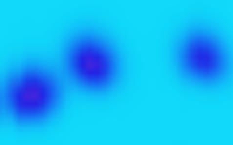
Each chemical in the sample produces a small blob or cluster of pixels with values that are larger than background values. The magnitudes of the pixel values indicate the quantity of the chemical present. Figure 1 illustrates a greatly magnified view of a small region of a GCxGC image containing three blobs of pixels indicating three separated chemicals. The smaller values of the background are colorized light-blue and the larger values of the blobs are colorized dark-blue and magenta.
The position (i.e., the retention times in each dimension) of each blob is related to the physical properties the chemical that produced the blob, so the position of a blob is useful in identifying each chemical in a sample. The sum of the pixel values in each blob is related to the quantity of the chemical that produced it, so the sum of pixel values of a blob is useful in quantifying each chemical in a sample. For a more extensive primer on comprehensive, two-dimensional gas chromatography, visit www.zoex.com.
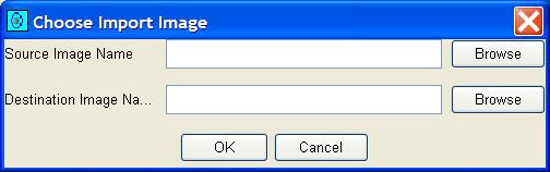
Specify the source and destination file names and click the OK
button. For example, a source file containing the raw data can be a text
file in comma-separated-value (CSV) format. The destination file name
is the name of the file to be created by GC Image. File system
browsers are available to help locate the files.
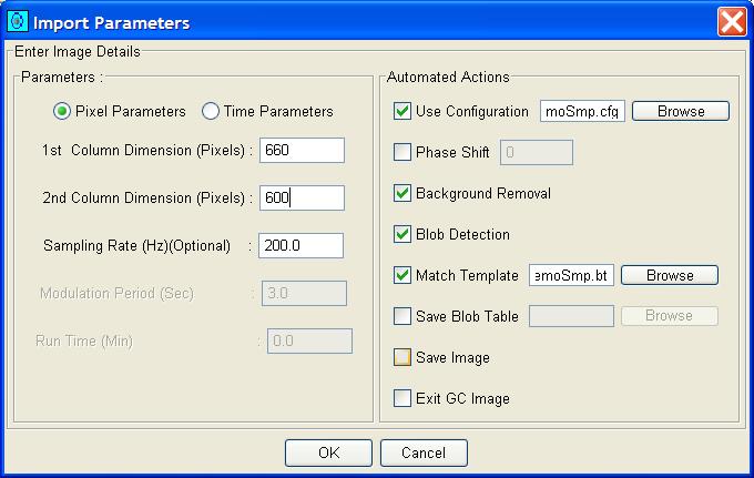
Specify the dimensions and optionally specify processing operations.
The dimensions of the data are required and may be given in pixel or
time units. For example, the dimensions of data acquired at 200 Hz
with a modulation period of 2 seconds and a run time of 20 minutes
could be sized equivalently as 600 pixels for the first dimension (20
minutes / 2 seconds/modulation) and 400 pixels for the second dimension
(200 samples/second * 2 seconds).
Specification of a configuration file and processing operations are
optional in this pop-up.
These optional specifications are a convenient mechanism for quickly
directing processing at the time data is imported.
Chapter Configuration Files
describes these capabilities. The rest of this quick tour demonstrates
how these operations are performed interactively.
Click the Correct Baseline button on the tool bar (a tool tip
is shown) or select Correct Baseline from the Filter menu.
To select blobs for inclusion, first set the cursor mode on the Image
Viewer palette to Select Blobs.
Subsequent chapters of the GC Image Users' Guide describe
installation and details on using the software.
Contents
Next: Installation and Start-Up
GC Image™ Users' Guide © 2001–2004 by GC Image, LLC, and
the University of Nebraska.
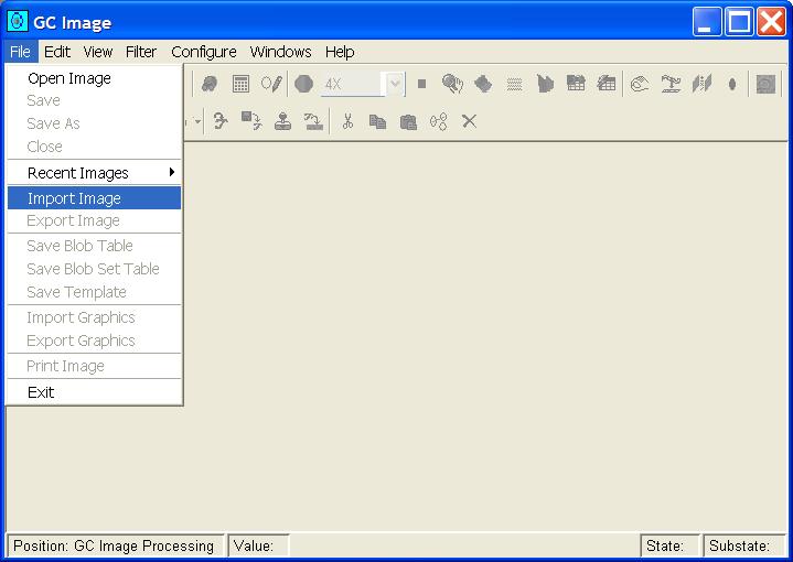
Step 1b: For the Import Image operation, GC Image
presents a popup dialog box for the source and destination file names.
Step 1c: After GC Image accepts the filenames, it presents a
popup dialog box for additional information about the image dimensions
and processing.
Step 1d: After the data is imported to form an image it is
displayed in the Image Viewer. A magnified region-of-interest
(ROI) is shown below. Here and in other figures, the GC Image interface
is resized to a small window for presentation.
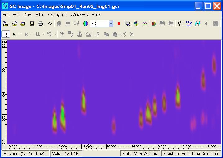
Step 2: This image has a background level of over 14 pico-amps.
(See the status bar below the image with the location of the cursor
and the data value at that pixel.) Before quantifying the blobs, the
baseline must be corrected.
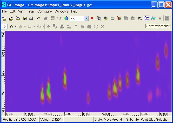
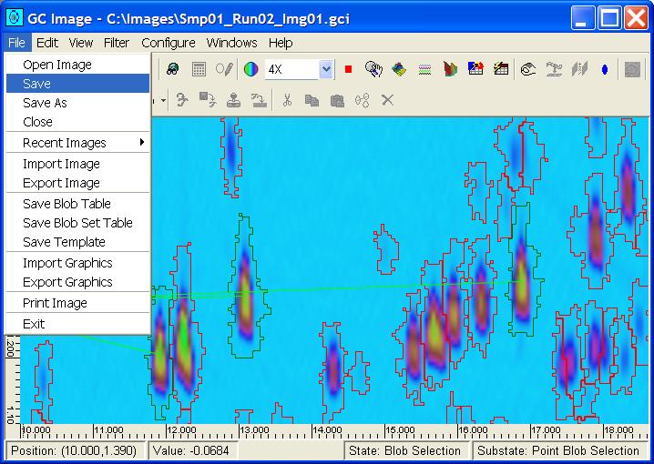
Step 3: After the baseline is corrected, note the change in
background value (indicated by the color change and by the value on
the status bar). Now, the blobs associated with the separated chemicals
can be detected and quantified. Press the Detect Blobs button
on the tool bar or select Detect Blobs from the Filter menu.
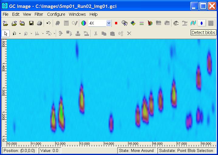
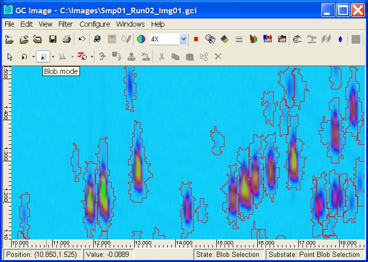
Step 4a: The blobs are detected and outlined. An image may
have thousands of blobs, but an analysis may require only a few of them.
Later sections of the GC Image Users' Guide explain how to use
template pattern matching to automatically identify and characterize
peaks of interest. Here, the quick tour shows interactive identification
and characterization.
Step 4b: Select a blob by positioning the cursor on the blob
and clicking the left mouse-button. The selected blob is graphically
highlighted with a colored box.
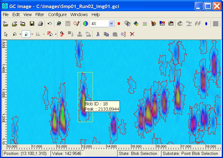
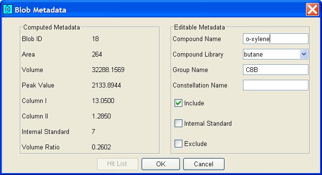
Step 4c: Once a blob is selected, click the right mouse-button to access a popup to view blob attributes and set blob metadata, including chemical name, group name, etc.
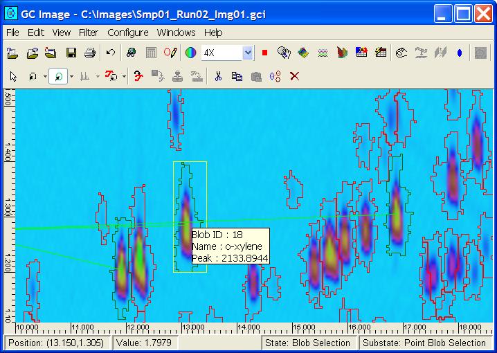
Step 4d: Graphical highlights show the included blobs, internal
standards, and associations between included blobs and internal
standards.
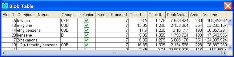
Step 4e: To view the Blob Table, press the Show Blob
Table button on the tool bar or select Show Blob Table from
the View menu. The Blob Table displays information about
each blob. The table can be sorted by clicking on a column header.
Step 5: Save the image with the Save (or Save As)
option from the File menu or by clicking the Save button
on the tool bar. Then exit with Exit from the File menu.